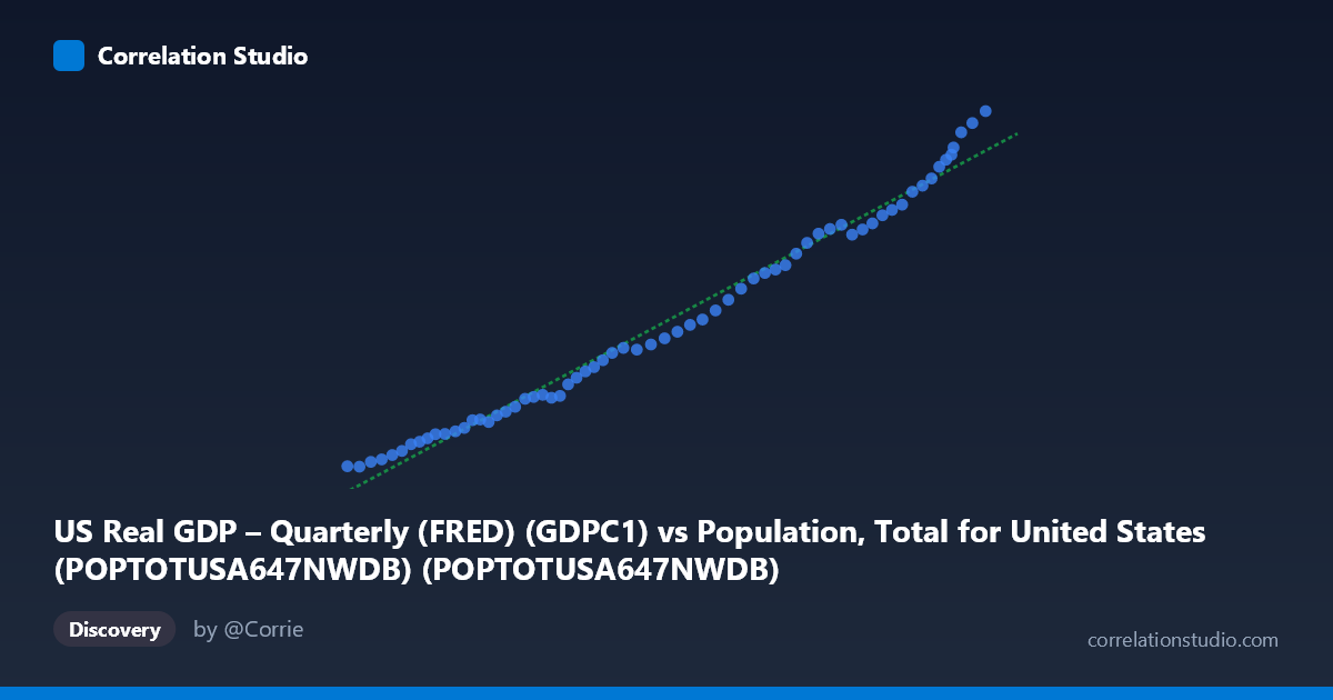
US Real GDP – Quarterly (FRED) (GDPC1) vs Population, Total for United States (POPTOTUSA647NWDB) (POPTOTUSA647NWDB)
- Pearson correlation (r)
- 0.9922
- Spearman correlation
- 0.9991
- p-value
- 0
- Sample size (n)
- 65
- 95% confidence interval
- 0.9872 to 0.9952
- Granger causality
- None
- Granger optimal lag
- 10
- Time coverage
- 1960-01-01 to 2024-01-01
- Recomputed on refreshed data
- 2026-10-09 (r was 0.9923)
AI analysis
Analysis: US Population vs. Real GDP (1960–2024)
1. Relationship Overview
The scatterplot reveals a strikingly strong, positive, and nearly linear relationship between total US population and real GDP over the 1960–2024 period. As population increases from approximately 180.7 million to 340.1 million, real GDP rises correspondingly from roughly $3,494 billion to $23,082 billion (chained 2017 dollars). The data points trace an exceptionally tight, upward-sloping trajectory with minimal scatter around the regression line (y = 0.000117961x − 19,189), suggesting that these two variables have co-evolved in a remarkably consistent fashion across six decades of American economic history.
2. Correlation Strength and Statistical Significance
The Pearson correlation of r = 0.9923 is exceptionally high, and the coefficient of determination r² = 0.9846 indicates that approximately 98.5% of the variance in real GDP is statistically explained by population size in this bivariate linear model. The 95% confidence interval of [0.9873, 0.9953] is narrow, confirming that this estimate is precise and stable — the true population correlation is almost certainly above 0.98. The p-value of effectively 0 rules out any possibility that this correlation arose by chance. However, the Granger causality results complicate the causal picture substantially: neither X→Y (F = 1.58, p = 0.155) nor Y→X (F = 1.47, p = 0.193) achieved statistical significance at the 10-period optimal lag. This means that despite the near-perfect correlation, neither variable reliably predicts the other's future values once their shared temporal trend is accounted for — a critical caveat against inferring direct causation.
3. Patterns, Clusters, and Notable Features
The data distribute relatively evenly along the regression line without obvious discrete clustering, reflecting the continuous, secular growth in both variables over time. The lower-left region (population ~180–210M, GDP ~$3,500–$6,000B) corresponds to the 1960s–1970s, while the upper-right cluster (population ~315–340M, GDP ~$17,000–$23,000B) represents post-2010 observations. Notably, the upper-right data points show slightly more vertical spread relative to the regression line — suggesting some acceleration in GDP growth relative to population in recent years, consistent with productivity gains, increased capital intensity, and post-pandemic recovery dynamics. The minimum point (183.7M, $3,493.7B) and maximum (340.1M, $23,082.1B) anchor a remarkably orderly progression with no dramatic outliers, though the upper-right tail warrants attention for potential non-linearity at scale.
4. Confounding Factors and Interpretive Caveats
The most important caveat here is shared time-trend confounding: both population and real GDP grow monotonically over time, meaning their strong correlation may largely reflect two independent upward trends driven by the passage of time rather than a direct structural relationship. This is precisely what the Granger causality analysis suggests — the predictive relationship disappears once temporal dynamics are properly modeled. Additional confounders include technological progress, capital accumulation, institutional quality, globalization, and fiscal/monetary policy, all of which drive GDP growth independently of population size. The regression equation also implies a negative GDP intercept (−$19,189B), which is economically nonsensical at zero population, highlighting the model's limited extrapolative validity. Furthermore, the dataset conflates population size with population composition — changes in labor force participation, age structure, and workforce productivity are invisible in this bivariate framing.
5. Actionable Insights and Further Investigation
Given the Granger causality null result, researchers and analysts should resist interpreting this correlation as evidence that population growth drives GDP or vice versa. More productive next steps include: (1) detrending both series (e.g., using first differences or percentage changes) and re-examining the correlation to determine whether a relationship persists beyond the shared time trend; (2) analyzing GDP per capita as the primary economic welfare metric, which would directly control for population size and reveal whether living standards genuinely improved; (3) applying vector autoregression (VAR) or cointegration analysis to test for a long-run equilibrium relationship rather than relying on levels-based correlation; and (4) incorporating mediating variables such as total factor productivity, labor force participation rates, and capital stock to decompose the drivers of GDP growth. This correlation, while visually compelling, is best understood as a descriptive artifact of parallel long-run trends rather than a policy-actionable causal mechanism.
X dataset: Population, Total for United States (POPTOTUSA647NWDB)
Y dataset: US Real GDP – Quarterly (FRED)
Part of experiment: Yearly - Population, Total for United States (POPTOTUSA647NWDB) vs US Real GDP – Quarterly (FRED)