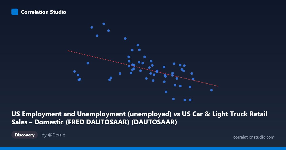
US Employment and Unemployment (unemployed) vs US Car & Light Truck Retail Sales – Domestic (FRED DAUTOSAAR) (DAUTOSAAR)
- Pearson correlation (r)
- -0.484
- Spearman correlation
- -0.4705
- p-value
- 0.000103
- Sample size (n)
- 59
- 95% confidence interval
- -0.6585 to -0.2601
- Granger causality
- None
- Granger optimal lag
- 10
AI analysis
Analysis: US Unemployment vs. Domestic Auto Retail Sales
Relationship Overview
The scatterplot reveals a moderate negative relationship between US unemployment levels and domestic auto retail sales (DAUTOSAAR). As unemployment increases, domestic auto sales tend to decline — a directionally intuitive finding, since higher unemployment typically suppresses consumer confidence and discretionary spending capacity. The linear regression equation (y = -615.57x + 11,482.8) quantifies this: each one-unit increase in the unemployment measure is associated with approximately 615 fewer units in annualized auto sales. However, the scatter around this regression line is substantial, indicating that unemployment alone is far from a complete explanation of auto sales dynamics across this 1967–2025 timeframe.
Correlation Strength, Direction, and Statistical Significance
The Pearson correlation of r = -0.484 confirms a moderate negative association, but the explained variance (r² = 0.234) tells a more sobering story: only about 23.4% of the variance in auto sales is explained by unemployment levels, leaving roughly 76.6% attributable to other factors. The 95% confidence interval for r ranges from -0.659 to -0.260, which, while entirely negative, is fairly wide — reflecting meaningful uncertainty in the precise magnitude of this relationship, partly a function of the paired sample size (n = 59). The p-value of 0.0001 confirms the correlation is statistically significant and highly unlikely to be a chance finding. However, the Granger causality tests are non-significant in both directions (X→Y: F = 2.08, p = 0.061; Y→X: F = 1.25, p = 0.306), meaning that — even at an optimal lag of 10 periods — neither variable reliably predicts the other temporally beyond what chance would suggest. This critically limits any causal narrative: correlation exists, but predictive temporal directionality does not hold up statistically.
Notable Patterns, Clusters, and Outliers
Several features stand out visually. There is a loose cluster of moderate-unemployment, moderate-sales points around the center of the distribution (X ≈ 5–8, Y ≈ 6,000–9,000), suggesting a regime of "normal" economic conditions. However, notable outliers strain the trend line significantly: - (3.62, 14,825) and (3.91, 13,747) represent very low unemployment paired with exceptionally high auto sales — consistent with boom-period dynamics - (2.90, 14,265) and (2.66, 8,623) show divergent outcomes at similarly low unemployment, suggesting other forces dominate at low unemployment extremes - (8.53, 2,817) and (8.85, 2,832) anchor the high-unemployment, low-sales corner, consistent with recessionary periods (likely 2008–2009 or early 1980s) - (2.07, 6,761) and (2.11, 5,996) are puzzling low-sales observations despite very low unemployment, potentially reflecting supply-side constraints (e.g., the 2021–2022 semiconductor shortage era)
The data also hints at possible non-linearity, particularly at the low-unemployment end where sales variance explodes, suggesting a threshold or regime-dependent relationship rather than a clean linear one.
Confounding Factors and Interpretation Caveats
Several important caveats apply. First, this analysis spans nearly six decades (1967–2025), during which the auto market, labor market definitions, consumer credit conditions, fuel prices, import competition, and vehicle types have changed dramatically — structural breaks likely exist within this time series. Second, unemployment as a single variable masks compositional differences: the same unemployment rate in 1982 vs. 2010 vs. 2023 reflects very different labor market conditions, wage dynamics, and consumer sentiment. Third, supply-side shocks (e.g., the 2021–2022 chip shortage reducing auto availability regardless of demand) can decouple sales from employment conditions entirely. Fourth, interest rates and auto financing costs — not captured here — are powerful mediators of auto purchase decisions. Finally, the annual aggregation of employment data paired with monthly auto sales rates may introduce temporal misalignment that obscures finer dynamics.
Actionable Insights and Further Investigation
Despite its limitations, this analysis offers meaningful starting points. Analysts should consider building a multivariate model incorporating consumer confidence indices, prime/auto loan interest rates, gasoline prices, and real disposable income alongside unemployment to substantially improve explained variance beyond the current 23.4%. Given the non-significant Granger causality, leading indicators other than unemployment (e.g., consumer sentiment surveys, credit availability metrics) may prove more predictively useful for auto sales forecasting. It would also be valuable to segment the time series into economic regimes (expansion vs. recession vs. supply-constrained periods) to test whether the unemployment–sales relationship is stronger or more causal within specific contexts. Finally, testing non-linear functional forms (quadratic or piecewise regression) could better capture the apparent heteroskedasticity at low unemployment levels and improve both model fit and interpretive accuracy.
X dataset: US Car & Light Truck Retail Sales – Domestic (FRED DAUTOSAAR)
Y dataset: US Employment and Unemployment
Part of experiment: Yearly - US Car & Light Truck Retail Sales – Domestic (FRED DAUTOSAAR) vs US Employment and Unemployment