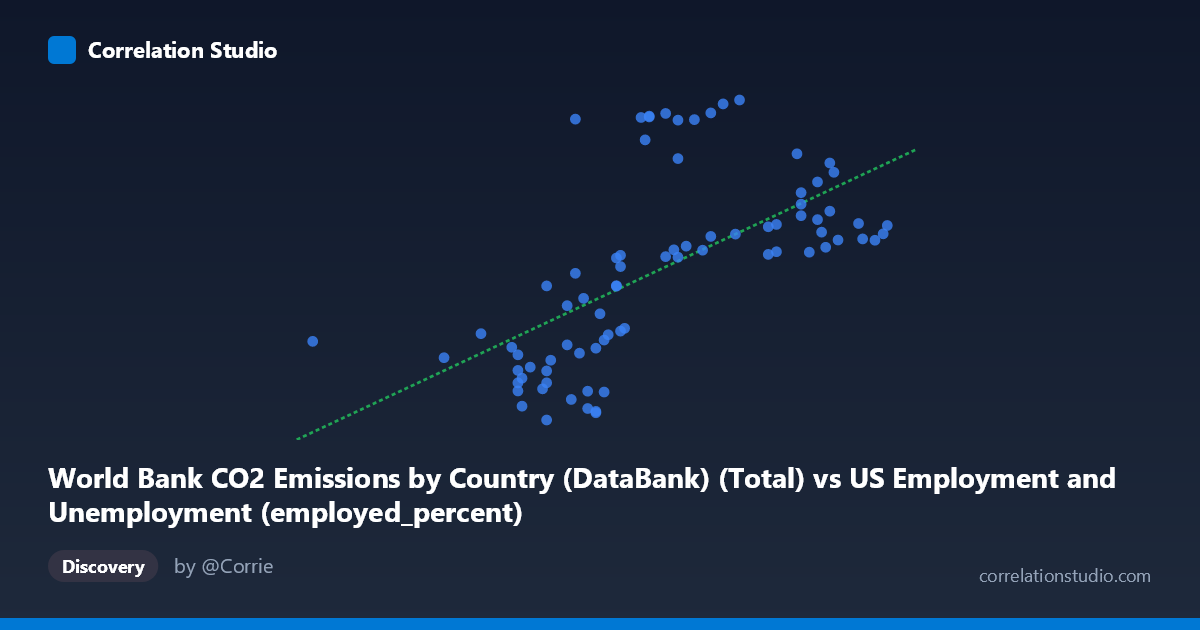
World Bank CO2 Emissions by Country (DataBank) (Total) vs US Employment and Unemployment (employed_percent)
- Pearson correlation (r)
- 0.6149
- Spearman correlation
- 0.7333
- p-value
- 0
- Sample size (n)
- 80
- 95% confidence interval
- 0.4569 to 0.7353
- Granger causality
- None
- Granger optimal lag
- 10
- Time coverage
- 1941-01-01 to 2020-01-01
AI analysis
Scatterplot Analysis: US Employment Rate vs. World Bank CO2 Emissions
1. Overall Relationship Revealed
The scatterplot depicts a positive association between a CO2 emissions total metric (X-axis, drawn from US employment/unemployment dataset context) and an employment percentage indicator (Y-axis, drawn from the World Bank CO2 dataset), spanning annual observations from 1941 to 2020. As X values increase across the range of roughly 50–65 units, Y values trend upward from approximately 10,000–20,000 toward 27,000–43,000. However, the scatter is notably wide, and the relationship is far from tight — points are dispersed broadly around the regression line (y = 1998.25x − 92,108.9), suggesting that while a general upward trend exists, many observations deviate substantially from linear expectation. The cross-dataset joining of these two variables (CO2 emissions and employment metrics from different primary sources) is an important structural note for interpretation.
2. Correlation Strength, Direction, and Temporal Causality
The Pearson correlation of r = 0.6149 indicates a moderate positive linear relationship, but the explanatory power is limited: R² = 0.3781, meaning only ~37.8% of the variance in Y is explained by X. Roughly 62% of Y's variation remains unexplained by this linear model alone. The 95% confidence interval of [0.457, 0.735] is moderately wide but does not cross zero, and the p-value of 1.30×10⁻⁹ confirms the correlation is highly statistically significant — making a chance finding extremely unlikely given n = 80. Critically, however, Granger causality analysis finds no significant predictive direction in either direction (X→Y: F = 1.02, p = 0.44; Y→X: F = 1.59, p = 0.14), meaning that past values of either variable do not significantly improve the prediction of the other's future values at any tested lag up to 10 periods. The statistical association is real, but temporal precedence — a prerequisite for causal inference — is absent.
3. Notable Patterns, Clusters, and Outliers
Several structural features stand out in the data:
- A horizontal band of high-Y outliers (Y ≈ 38,000–43,000) appears across a wide range of X values (~56–61), including points like (56.80, 41,141), (58.40, 41,311), (59.70, 41,089), and (60.80, 43,129). These observations break the linear trend dramatically and suggest a distinct sub-population or regime in the data. - A lower-left cluster of low X, low Y values (X ≈ 53–58, Y ≈ 10,000–17,000) forms a relatively tight grouping consistent with earlier time periods or different economic/emissions contexts. - The note that Spearman ρ exceeds Pearson r is a meaningful diagnostic — it suggests the true relationship may be monotonic but non-linear, potentially better described by a polynomial or logarithmic curve. This is visually consistent with the apparent "fanning" or acceleration of Y values at higher X. - The point (50.40, 18,044) is an isolated low-X outlier with a surprisingly mid-range Y value, pulling against the trend.
4. Confounding Factors and Interpretive Caveats
This correlation carries substantial interpretive risk for several reasons:
- Cross-dataset joining: The X variable comes from an employment dataset labeled as a CO2 total, and the Y variable comes from a CO2 dataset labeled as an employment percentage. This column-label mismatch suggests a database join artifact — these may not be organically paired time series, raising the possibility of spurious correlation by construction. - Temporal confounding: Both CO2 emissions and employment rates share a common driver — long-run economic growth. Over 80 years (1941–2020), both series would be expected to trend upward together due to GDP expansion, population growth, and industrialization, regardless of any direct link. This is a classic common-trend spurious correlation. - Structural breaks: The 1941–2020 window spans World War II, postwar expansion, oil crises, deindustrialization, and COVID-19 — each introducing regime shifts that could artifically cluster data and inflate or deflate correlation. - Aggregation level: "Total" CO2 at the country level is a macro aggregate; employment percent is a ratio. These operate at different scales and may not represent comparable units of analysis for causal reasoning.
5. Actionable Insights and Further Investigation
Given the moderate but non-causal correlation and visible non-linearity, the following steps are recommended:
1. Detrend both series (e.g., first-differencing or HP filter) before computing correlations to remove shared secular trends and test whether the relationship persists beyond common growth trajectories. 2. Fit a polynomial or logarithmic regression model, as suggested by Spearman ρ Pearson r, and compare AIC/BIC to the linear model to determine if a better functional form exists. 3. Investigate the high-Y cluster (~38,000–43,000) separately — these may correspond to specific decades (likely postwar boom or late 20th century) and may warrant segmented analysis. 4. Validate the dataset join logic to confirm that X and Y represent genuinely co-occurring annual measurements for the same country/year, not an artifact of a misaligned merge key. 5. Include GDP, population, and energy intensity as covariates in a multivariate model to partial out confounders and isolate any residual direct association between emissions and employment.
X dataset: US Employment and Unemployment
Y dataset: World Bank CO2 Emissions by Country (DataBank)
Part of experiment: Yearly - US Employment and Unemployment vs World Bank CO2 Emissions by Country (DataBank)