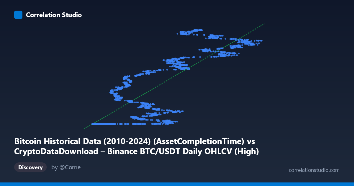
Bitcoin Historical Data (2010-2024) (AssetCompletionTime) vs CryptoDataDownload – Binance BTC/USDT Daily OHLCV (High)
- Pearson correlation (r)
- 0.85
- Spearman correlation
- 0.886
- p-value
- 0
- Sample size (n)
- 3191
- 95% confidence interval
- 0.8401 to 0.8593
- Granger causality
- None
- Granger optimal lag
- 10
AI analysis
Analysis: BTC Completion Time Metric vs. BTC/USDT Daily High Price
1. What the Visualization Reveals
This scatterplot compares a column labeled "Asset Completion Time" against the daily "High" price of BTC/USDT on Binance. Despite the axis label, the X variable's behavior strongly suggests it is not a timestamp in the conventional sense but rather a derived or transformed value (ranging ~3,276–126,200) that correlates with price levels. The data shows a clear non-linear, step-like structure: a dense cluster of points near X≈3,000–20,000 sits flat at Y≈1,614,337,000–1,614,338,000 (essentially a constant "floor" value), while points with X 20,000 fan out across a much wider Y range (1,617M–1,779M), rising roughly in tandem with X. This bifurcated pattern — a flat plateau followed by a rising trend — is the dominant visual feature, not a smooth linear cloud.
2. Strength, Direction, and Statistical Confidence
The Pearson correlation (r = 0.85, r² = 0.72) indicates a strong positive linear association, with 72% of the variance in Y statistically explained by X. The tight confidence interval [0.840, 0.859] and p-value of 0 confirm this relationship is highly stable and not a product of sampling noise — with n = 3,191, even modest correlations would be significant, so the effect size here is meaningful, not just statistically detectable. However, the Granger causality tests tell a different story: neither direction (X→Y or Y→X) shows significant predictive power (p = 0.31 and p = 0.13 respectively) at the optimal lag of 10 periods. This is a critical distinction: strong contemporaneous correlation does not imply that one variable temporally leads or forecasts the other. Practically, this means you cannot use past values of X to predict future Y (or vice versa) with this model — the relationship is likely driven by both variables reflecting a shared underlying process (e.g., both tracking overall market growth/time progression) rather than one causing the other.
3. Notable Patterns and Non-Linear Features
The most striking feature is the flat plateau for low X values (~3,000–20,000), where Y is pinned near its minimum (~1,614,337,000) regardless of X's variation within that range — this looks like a floor/clipping effect, a placeholder value, or an artifact of how "completion time" is encoded for early/incomplete records. Beyond this plateau, the relationship becomes much more scattered and heteroscedastic, with increasing variance in Y as X grows (e.g., at X≈84,000, Y ranges from 1,741M to 1,778M). This fan-shaped spread suggests the linear model (y = 1403.99x + 1.61E9) fits the aggregate trend but poorly captures the two distinct regimes — a piecewise or log-transformed model would likely fit better.
4. Confounding Factors and Caveats
Several concerns limit interpretation: (1) The X-axis semantics are unclear — "Asset Completion Time" is an unusual pairing with a price series, and the flat plateau suggests it may encode something like row-processing order, an index, or a time-since-event metric rather than a true independent variable. (2) Both series likely share a common trend driver: Bitcoin's price has risen dramatically from 2017–2026, so any monotonically increasing X (even an arbitrary counter) will spuriously correlate with Y. (3) The data are highly autocorrelated time series (daily OHLCV), violating the independence assumption behind standard r and p-value calculations — the "N=3,212 vs n=3,191" gap and daily granularity mean effective degrees of freedom are likely far lower than reported, inflating apparent significance.
5. Actionable Next Steps
1. Clarify the X variable's definition — verify whether "Asset Completion Time" is a genuine timestamp, an index, or a derived metric; the plateau behavior is a red flag warranting investigation. 2. Segment the analysis by the two visible regimes (plateau vs. rising trend) and fit separate models, or apply a log/spline transform to X. 3. Test for a shared trend/unit-root — run cointegration tests or difference both series before correlating, since both likely trend with calendar time independently. 4. Do not use this relationship for forecasting — the null Granger causality result means neither variable should be used to predict the other's future values; treat r² as descriptive of co-movement only. 5. Investigate the plateau cluster as a potential data quality issue (missing values, default fills, or truncated timestamps) before drawing further conclusions.
X dataset: CryptoDataDownload – Binance BTC/USDT Daily OHLCV
Y dataset: Bitcoin Historical Data (2010-2024)
Part of experiment: Bitcoin - CryptoDataDownload – Binance BTC/USDT Daily OHLCV vs Bitcoin Historical Data (2010-2024)