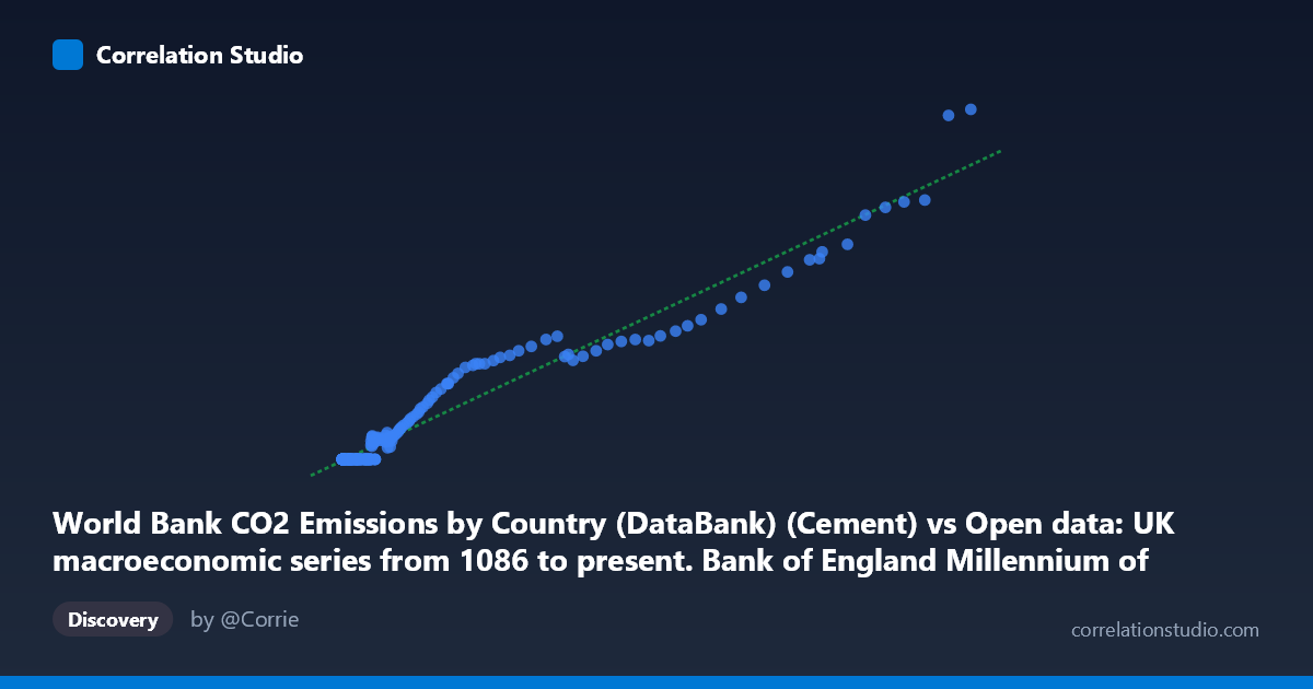
World Bank CO2 Emissions by Country (DataBank) (Cement) vs Open data: UK macroeconomic series from 1086 to present. Bank of England Millennium of Macroeconomic Data. (Year) (value)
- Pearson correlation (r)
- 0.9791
- Spearman correlation
- 0.8327
- p-value
- 0
- Sample size (n)
- 266
- 95% confidence interval
- 0.9735 to 0.9836
- Granger causality
- Y → X
- Granger optimal lag
- 10
- Time coverage
- 1751-01-01 to 2016-01-01
AI analysis
Analysis of UK Macroeconomic Data vs. Global Cement CO₂ Emissions
1. Overall Relationship The scatterplot reveals a striking positive relationship between World Bank cement CO₂ emissions (X-axis) and a UK macroeconomic indicator from the Bank of England's Millennium dataset (Y-axis). The data spans an extraordinary temporal range (1751–2016), capturing the full arc of industrialization. The linear regression equation (y = 0.00430x − 18.82) fits the data remarkably well across a wide dynamic range — from near-zero values clustering at the origin to extreme values exceeding 350,000 kt of cement CO₂ paired with macroeconomic readings above 1,300. The relationship appears largely linear through much of its range, with the scatter tightening at lower values and widening modestly at higher ones, suggesting slight heteroscedasticity.
2. Correlation Strength and Statistical Significance The correlation is exceptionally strong (r = 0.9791), and critically, R² = 0.9587 means that 95.9% of the variance in the UK macroeconomic indicator is statistically explained by variation in cement CO₂ emissions. The 95% confidence interval [0.9735, 0.9836] is narrow, confirming this is not an artifact of small sample uncertainty, and the p-value of effectively zero (against N = 18,769) makes this correlation statistically indisputable. However, the Granger causality results introduce an important directional nuance: Y Granger-causes X (F = 2.02, p = 0.032), while X does not significantly Granger-cause Y (F = 1.51, p = 0.137). This means the UK macroeconomic variable has temporal predictive power over cement emissions — not the reverse — suggesting the economic variable leads the emissions signal by approximately 10 periods (years), consistent with the idea that economic activity precedes industrial output.
3. Notable Patterns, Clusters, and Outliers The sample points reveal a pronounced lower-left cluster — roughly half the sampled observations have Y = 0.00 despite non-trivial X values (e.g., X ≈ 2,000–25,000), indicating a floor effect or censoring in the macroeconomic series for earlier historical periods. This bimodal character (zeros vs. continuous positive values) is a significant structural feature. At the upper end, several points (e.g., X ≈ 356,380 / Y ≈ 1,362; X ≈ 298,265 / Y ≈ 1,099) sit along the regression line without appearing as dramatic outliers, suggesting the linear model holds well at extremes. The moderate scatter in the mid-range (X: 50,000–200,000) points to periods of decoupling — likely wartime disruptions, recessions, or energy transitions — where the two series temporarily diverge.
4. Confounding Factors and Interpretive Caveats This correlation almost certainly reflects shared trending with time rather than a direct causal mechanism between UK macroeconomics and global cement emissions. Both series grow monotonically over centuries driven by the same underlying force: global industrialization and economic development. This is a classic case of spurious correlation via common temporal trend — two independently rising time series will correlate strongly regardless of any mechanistic link. The zero-floor values in Y for early periods further suggest data availability gaps rather than true zeros, which artificially compresses variance in one direction. The Granger result, while nominally significant, operates at a 10-year lag across a non-stationary series, and without differencing or cointegration testing, the result may be unreliable. The mismatch in dataset descriptions (axis labels appear swapped in the metadata) also warrants careful verification before drawing conclusions.
5. Actionable Insights and Further Investigation Before treating this correlation as meaningful, detrending both series (first-differencing or HP filtering) is essential to remove shared secular growth trends and test whether the relationship persists in stationary form. Researchers should: (a) apply cointegration tests (Engle-Granger or Johansen) to determine whether any long-run equilibrium relationship exists beyond shared trending; (b) investigate the structural breaks visible in the mid-range scatter, potentially corresponding to WWI/WWII, the 1970s oil crises, or the 2008 financial crisis; (c) verify the axis label alignment given the metadata inconsistency between X and Y dataset descriptions; and (d) expand the Granger analysis using VAR models with differenced data to produce reliable directional inference. If the relationship survives detrending, the 10-year Granger lead of UK macroeconomics over cement emissions could have genuine forecasting utility for industrial emissions projections.
X dataset: Open data: UK macroeconomic series from 1086 to present. Bank of England Millennium of Macroeconomic Data. (Year)
Y dataset: World Bank CO2 Emissions by Country (DataBank)
Part of experiment: Yearly - Open data: UK macroeconomic series from 1086 to present. Bank of England Millennium of Macroeconomic Data. (Year) vs World Bank CO2 Emissions by Country (DataBank)