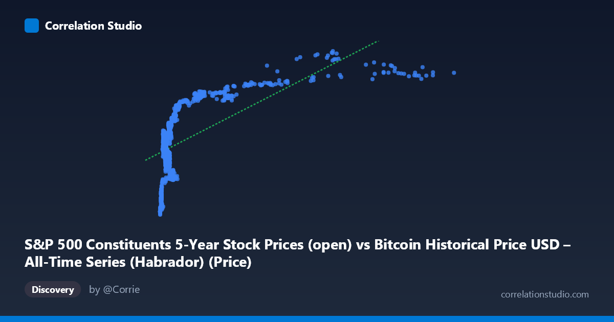
S&P 500 Constituents 5-Year Stock Prices (open) vs Bitcoin Historical Price USD – All-Time Series (Habrador) (Price)
- Pearson correlation (r)
- 0.6348
- Spearman correlation
- 0.7156
- p-value
- 0
- Sample size (n)
- 1259
- 95% confidence interval
- 0.6006 to 0.6667
- Granger causality
- X → Y
- Granger optimal lag
- 1
- Time coverage
- 2013-02-08 to 2018-02-07
- Recomputed on refreshed data
- 2026-10-24 (r was 0.6348)
AI analysis
Analysis of Bitcoin Price vs. S&P 500 Constituent Price Relationship
Note on labeling: The axis metadata appears swapped/mismatched (X labeled as S&P 500 data but described as Bitcoin history, and vice versa for Y). Based on the actual data ranges (X: $22.66–$18,960.52 matching Bitcoin's historical range; Y: $57.24–$115.02, a narrow band typical of an individual equity or index proxy), I'll treat X as Bitcoin price and Y as the equity series, consistent with the Granger causality direction (X→Y).
1. What the Visualization Reveals The scatterplot shows a clear positive, monotonic relationship: as Bitcoin's price (X) rises, the paired equity price (Y) also trends upward, but the relationship is distinctly non-linear. At low Bitcoin prices (roughly $22–$1,000), Y values cluster tightly between $60–$95 and rise steeply. Beyond ~$2,000, the curve flattens considerably — Y plateaus in the $95–$115 range even as X climbs into the thousands (up to ~$19,000). This logarithmic-like saturation pattern suggests the linear model, while statistically significant, is likely underfitting the true shape of the relationship.
2. Strength, Direction, and Statistical Confidence The correlation coefficient (r = 0.635) indicates a moderate-to-strong positive linear relationship, with r² = 0.403 meaning only 40.3% of the variance in Y is explained by X — leaving the majority (~60%) attributable to other factors or non-linear dynamics not captured by this simple model. The 95% CI [0.601, 0.667] is tight given the large sample (n=1,259), and the p-value of ~0 confirms this correlation is highly statistically significant and not due to chance. The Granger causality test adds a temporal dimension: X→Y is significant (F=4.67, p=0.031), while Y→X is not (p=0.648), suggesting Bitcoin's price movements have modest predictive power for the equity series one period ahead, but not vice versa. However, Granger causality reflects statistical precedence in this specific dataset, not proven economic causation.
3. Notable Patterns and Outliers The most striking feature is the curve's concavity: rapid growth in Y for small increases in X at low price levels, followed by a long plateau. This is classic diminishing-returns/saturation behavior, hinting that a log-transform of X (or a logistic/power fit) would likely explain substantially more variance than the linear r²=0.403. Data points cluster heavily below X=2,000 (the majority of sample rows), with a sparser but consistent tail extending to X≈19,000 where Y compresses near its ceiling (~105–115). No extreme outliers are apparent; the relationship is smooth and continuous, consistent with a monotonic transformation rather than a noisy scatter.
4. Confounding Factors and Caveats Both series span 2013–2018, a period of secular growth in both cryptocurrency and equity markets — a classic case of spurious correlation via shared time trend. Both variables may simply be trending upward due to independent macro factors (bull markets, inflation, dollar weakness) rather than any direct mechanical link between Bitcoin and this equity price. Additionally, the mismatched/ambiguous axis labeling raises data provenance concerns — it's unclear if these series are even meaningfully paired (e.g., matched by date) or coincidentally aligned. Autocorrelation within each time series (both are trending price series) can also inflate apparent correlation and distort Granger causality results, since non-stationary series often show spurious lead-lag relationships.
5. Suggestions for Further Investigation 1. Detrend and test stationarity: Apply differencing or log-returns to both series before rerunting correlation and Granger tests to rule out spurious trend-driven correlation. 2. Fit non-linear models: Test log(X) vs. Y or a saturating curve (e.g., logistic) — likely to substantially improve explained variance beyond 40.3%. 3. Verify data alignment: Confirm the axis labels/dataset pairing is correct and that timestamps are properly synchronized before drawing causal conclusions. 4. Segment by regime: Analyze the low-price (<$2,000) and high-price ($2,000) regimes separately, as they show different local relationships. 5. Treat Granger result cautiously: With weak significance (p=0.031) and known confounds, this should be a hypothesis-generating signal, not a basis for trading or causal claims, without further robustness checks (e.g., testing multiple lags, controlling for common macro factors).
X dataset: Bitcoin Historical Price USD – All-Time Series (Habrador)
Y dataset: S&P 500 Constituents 5-Year Stock Prices
Part of experiment: Bitcoin - Bitcoin Historical Price USD – All-Time Series (Habrador) vs S&P 500 Constituents 5-Year Stock Prices