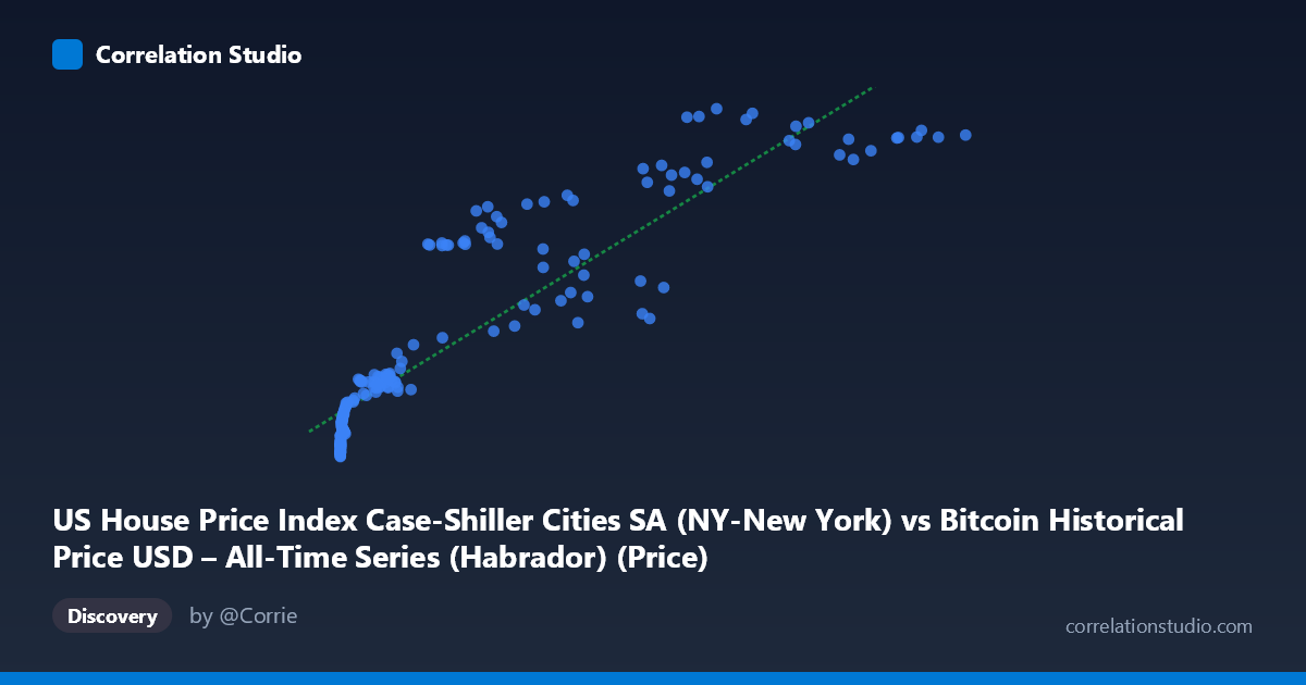
US House Price Index Case-Shiller Cities SA (NY-New York) vs Bitcoin Historical Price USD – All-Time Series (Habrador) (Price)
- Pearson correlation (r)
- 0.905
- Spearman correlation
- 0.9625
- p-value
- 0
- Sample size (n)
- 187
- 95% confidence interval
- 0.8751 to 0.928
- Granger causality
- None
- Granger optimal lag
- 1
AI analysis
Analysis: Bitcoin Price vs. NY Case-Shiller Home Price Index
1. Relationship Overview
The scatterplot depicts a strongly positive, monotonic but distinctly non-linear relationship between Bitcoin's USD price (X) and the NY Case-Shiller Home Price Index (Y). The data traces a classic diminishing-returns curve: Y rises steeply as X moves from near-zero to roughly 1,000, then flattens considerably as X climbs into the tens of thousands and beyond. This shape is typical when a highly right-skewed variable (Bitcoin price, ranging from $0.06 to $118,670, spanning nearly 7 orders of magnitude) is plotted against a comparatively narrow-range, slow-moving variable (the housing index, 160–341).
2. Strength, Direction, and Statistical Caveats
The linear correlation is strong (r = 0.905, R² = 0.819), meaning a simple linear model explains about 82% of the variance in Y. The 95% CI [0.875, 0.928] is tight and the p-value is effectively 0, so the correlation is highly unlikely to be a sampling artifact. However, strength of correlation should not be conflated with causal linkage or mechanistic connection — and the Granger causality tests confirm this directly: neither direction shows significant predictive power (X→Y: p=0.357; Y→X: p=0.212). This means that despite the high contemporaneous correlation, Bitcoin price changes do not statistically precede/predict housing index changes, nor vice versa, at the tested lag. This is a strong signal that the correlation is driven by both series independently trending upward over the same historical period (2010–2026) rather than one influencing the other through any time-lagged mechanism.
3. Notable Patterns and Outliers
Several features stand out: - Compressed origin cluster: The vast majority of points sit at very low X values (sub-$1,000, in fact many under $100) corresponding to Bitcoin's early years, where Y ranges narrowly from ~160 to ~200. This creates a dense cluster near the origin that dominates the point count but contributes little to the visual spread. - Sparse high-X tail: Only a handful of points exist above X = 40,000, representing Bitcoin's 2020s bull-market prices; these carry disproportionate leverage in the regression fit. - Curvature/heteroscedasticity: The relationship visibly saturates — Y increases much more slowly per unit X at high Bitcoin prices than at low ones, suggesting a logarithmic or power-law fit (e.g., Y ~ log(X)) would likely outperform the linear model (R²=0.819) and reduce residual patterns. - No extreme outliers are apparent; the fit residuals seem consistent with the curvature rather than isolated anomalies.
4. Confounding Factors and Caveats
This is a classic case of two independent trending time series being compared, where the shared timeframe (2010–2026) itself is the primary confound. Both Bitcoin's price and US home prices experienced substantial secular growth over this period due to entirely different drivers — Bitcoin due to adoption/speculation cycles, housing due to macroeconomic factors (interest rates, wage growth, supply constraints, monetary policy, post-COVID demand shifts). A shared macro backdrop (e.g., loose monetary policy, low interest rates 2010–2021, inflation post-2021) could induce spurious correlation between any two upward-trending series over this window, and this is highly likely here. The mismatched sample sizes (N=470 population vs. n=187 paired sample) also warrant checking how the subsample was selected, as this could introduce bias.
5. Actionable Insights
- Do not interpret this as a causal or tradeable relationship — the lack of Granger causality strongly argues against using Bitcoin price to predict housing index moves or vice versa. - Refit with a log transform on X (and possibly Y) to better capture the true functional form and get a more honest R² and residual diagnostic. - Detrend both series (e.g., using differences or growth rates rather than levels) and recheck correlation/Granger causality; this is the standard remedy for spurious correlation between trending series and would likely show the correlation collapse substantially. - Investigate shared macro covariates (interest rates, CPI, M2 money supply) as a more plausible common driver than any direct linkage between crypto and regional housing markets.
X dataset: Bitcoin Historical Price USD – All-Time Series (Habrador)
Y dataset: US House Price Index Case-Shiller Cities SA
Part of experiment: Bitcoin - Bitcoin Historical Price USD – All-Time Series (Habrador) vs US House Price Index Case-Shiller Cities SA