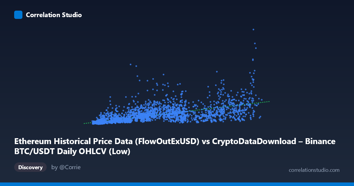
Ethereum Historical Price Data (FlowOutExUSD) vs CryptoDataDownload – Binance BTC/USDT Daily OHLCV (Low)
- Pearson correlation (r)
- 0.6508
- Spearman correlation
- 0.8185
- p-value
- 0
- Sample size (n)
- 3191
- 95% confidence interval
- 0.6304 to 0.6704
- Granger causality
- Y → X
- Granger optimal lag
- 10
AI analysis
Analysis: Ethereum FlowOutExUSD vs. BTC/USDT Low Price
1. What the Visualization Reveals
The scatterplot shows a moderate positive relationship between X (labeled as Ethereum FlowOutExUSD, though the range/scale strongly suggests this is mislabeled and behaves like a transaction-count or volume-adjusted metric) and Y (BTC/USDT daily low price). As X increases from its minimum (~2,817) to its maximum (~123,084), Y trends upward from the tens of millions into the billions range. However, the relationship is clearly not tight — there is substantial vertical scatter at every X value, indicating that X alone is a weak-to-moderate predictor of Y's exact value.
2. Strength, Direction, and Statistical Confidence
The Pearson correlation (r = 0.6508) indicates a moderate positive linear relationship. Squaring this, r² = 0.4236 tells us that only 42.4% of the variance in Y is explained by X — meaning more than half the variability in BTC's low price is driven by factors outside this X variable entirely. The 95% CI [0.6304, 0.6704] is tight and does not cross zero, and with p ≈ 0 across n=3,191 points, we can be highly confident a real (non-zero) linear association exists — this is not a statistical fluke, but it is also not a strong deterministic relationship.
The Granger causality results add an important temporal dimension: Y Granger-causes X, not the other way around (F=2.07, p=0.024 for Y→X vs. F=1.47, p=0.145 for X→Y, not significant). This suggests that past values of BTC price (Y) have predictive power over future values of X, at a lag of 10 periods — the reverse is not supported. Practically, this implies X should not be treated as a leading indicator for BTC price movements; if anything, BTC price history helps predict X.
3. Notable Patterns and Non-linearity
The regression line (y = 12,997.7x + 91.87M) fits reasonably but the note that Spearman ρ exceeds Pearson r is a key signal: the relationship is monotonic but likely curved rather than linear — plausibly logarithmic or power-law, which is common when comparing a bounded/count-like metric (X) against price levels (Y) that span nearly three orders of magnitude (13.9M to 7.36B). Looking at the sample points, there are clusters of high-Y/low-to-mid-X pairs (e.g., X≈35,440 with Y≈1.3B, X≈56,691 with Y≈1.69B) alongside many low-X/low-Y pairs clustered below X=15,000 and Y<300M — suggesting heteroscedasticity (variance in Y grows with X) and possibly two overlapping regimes or market cycles (e.g., bull vs. bear market periods) rather than one continuous trend.
4. Confounding Factors and Caveats
Several caveats are essential here: - Metadata mismatch: The axis labels are confusing/likely mislabeled (X is described as an Ethereum "FlowOutExUSD" column but sourced from Binance BTC/USDT OHLCV data; Y is BTC low price sourced from an "Ethereum" dataset). This cross-labeling raises real concern about whether the plotted variables are what they claim to be — verify column mapping before drawing conclusions. - Time-series autocorrelation: Both series span 2017–2026 and are almost certainly non-stationary (trending) daily data. Standard Pearson r and even Granger tests on non-stationary series can produce spurious or inflated results unless the data were differenced or detrended — this is a major caveat given crypto's well-known long-term uptrends. - Shared macro drivers: BTC and ETH-related metrics are both driven by common crypto-market-wide factors (liquidity cycles, regulatory news, macro risk sentiment), so correlation likely reflects shared exposure to market cycles rather than a direct causal link between the two specific variables.
5. Actionable Insights
1. Verify data provenance/labels — resolve the apparent mismatch between column descriptions and dataset sources before using this for any modeling or trading decisions. 2. Test log-transformed or polynomial models — given the Spearman/Pearson divergence and Y's multi-order-of-magnitude range, refit using log(Y) ~ X or log(Y) ~ log(X) to likely improve fit substantially beyond 42% variance explained. 3. Check stationarity — run ADF/KPSS tests and consider differencing both series before trusting the Granger causality direction, since trending series can produce misleading lag-predictive signals. 4. Segment by market regime — split the data by bull/bear periods or by year to check if the relationship strength/direction is stable over time or is an artifact of a few high-volatility periods (e.g., 2021 bull run, 2022 crash). 5. Use Y→X finding cautiously — if confirmed robust after detrending, this suggests BTC price history may have modest forecasting value for the X metric at a ~10-period lag, worth exploring further with out-of-sample validation rather than relying on the reverse assumption.
X dataset: CryptoDataDownload – Binance BTC/USDT Daily OHLCV
Y dataset: Ethereum Historical Price Data
Part of experiment: Bitcoin - CryptoDataDownload – Binance BTC/USDT Daily OHLCV vs Ethereum Historical Price Data