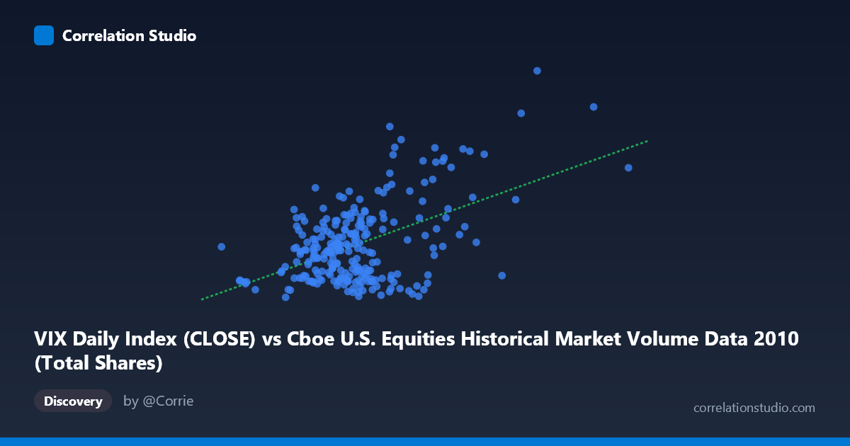
VIX Daily Index (CLOSE) vs Cboe U.S. Equities Historical Market Volume Data 2010 (Total Shares)
- Pearson correlation (r)
- 0.4969
- Spearman correlation
- 0.2639
- p-value
- 0
- Sample size (n)
- 252
- 95% confidence interval
- 0.3978 to 0.5846
- Granger causality
- Y → X
- Granger optimal lag
- 1
- Time coverage
- 2010-01-04 to 2010-12-31
- Recomputed on refreshed data
- 2026-10-09 (r was 0.4969)
AI analysis
Analysis: VIX vs. U.S. Equity Market Volume (2010)
Relationship Overview The scatterplot reveals a moderate positive relationship between U.S. equity market trading volume (X-axis) and the CBOE Volatility Index (VIX, Y-axis) across 252 trading days in 2010. As market volume increases, VIX levels tend to rise as well, which aligns intuitively with market microstructure theory: elevated volatility typically drives heightened trading activity as investors reposition, hedge, or react to uncertainty. The linear regression equation (y = 1.37×10⁻⁸x + 13.52) suggests that for every additional ~73 million shares traded, VIX rises by approximately 1 point, with a baseline VIX of ~13.5 at minimal volume.
Correlation Strength and Statistical Significance The Pearson correlation of r = 0.497 indicates a moderate positive association, but the more telling statistic is r² = 0.247, meaning only about 24.7% of the variance in VIX is explained by trading volume. The remaining ~75% is driven by factors not captured in this bivariate model. The 95% confidence interval of [0.398, 0.585] is reasonably narrow given the sample size (n=252), and the p-value of effectively zero confirms this relationship is statistically robust — not a sampling artifact. Critically, the Granger causality analysis points unidirectionally: VIX Granger-causes volume (F=6.46, p=0.012), while volume does not significantly predict VIX (F=2.36, p=0.126). This temporal ordering is practically meaningful — rising fear/volatility expectations appear to precede trading surges, rather than the reverse. Markets seem to respond to volatility signals rather than generate them through volume alone.
Notable Patterns, Clusters, and Outliers The scatterplot exhibits several notable structural features. The bulk of observations cluster in a lower-left region (volume ~400M–800M shares, VIX ~15–25), suggesting most of 2010 was characterized by moderate, relatively calm trading conditions. However, there is a visible upper-right dispersion of high-volume, high-VIX days that stretches the relationship. Several prominent outliers stand out: one point near (1,476,963,723; 40.95) and another near (1,225,972,710; 40.10) represent extreme combinations of volume and volatility, likely corresponding to crisis episodes such as the May 2010 Flash Crash or European sovereign debt contagion events. Point (771,053,019; 38.32) also stands apart. Additionally, there are counter-intuitive observations — high-volume days with low VIX (e.g., ~888M shares at VIX 16.47) and moderate-volume days with elevated VIX — suggesting the relationship is heteroscedastic and non-linear at the extremes, with variance in VIX expanding substantially as volume increases.
Confounding Factors and Caveats Several important caveats temper interpretation. First, reverse causality and simultaneity are difficult to fully disentangle even with Granger tests — both variables are reflexively tied to market sentiment, macro news, and institutional behavior. Second, temporal autocorrelation is almost certainly present in both daily VIX and volume series, which can inflate apparent correlations; the Granger framework partially addresses this but doesn't eliminate it. Third, structural breaks — particularly the Flash Crash of May 6, 2010 — likely disproportionately influence both the regression slope and the outlier cluster, and their removal might substantially alter the estimated relationship. Fourth, the axis labels appear swapped relative to convention (VIX is on the Y-axis but labeled as the X dataset source, and vice versa), which warrants verification of the data mapping before drawing firm conclusions. Finally, 2010 represents a specific macro regime (post-GFC recovery, European debt crisis) that may not generalize to other periods.
Actionable Insights and Further Investigation Practitioners monitoring equity markets could use VIX as a leading indicator for volume surges with a 1-day lag, which has direct implications for liquidity management, transaction cost forecasting, and execution strategy — high-VIX environments may warrant adjusted order sizing or timing. For further investigation, it would be valuable to: (1) segment the analysis by market regimes (e.g., calm vs. stress periods) to test whether the correlation strengthens non-linearly above VIX thresholds like 25 or 30; (2) apply a log transformation to volume to address heteroscedasticity and potentially improve model fit; (3) test a multivariate model incorporating additional predictors (e.g., S&P 500 returns, bid-ask spreads, options open interest) to capture more of the unexplained 75% variance; and (4) validate Granger causality across multiple years to confirm whether the VIX→Volume predictive relationship is stable or regime-dependent.
X dataset: Cboe U.S. Equities Historical Market Volume Data 2010
Y dataset: VIX Daily Index
Part of experiment: Daily - Cboe U.S. Equities Historical Market Volume Data 2010 vs VIX Daily Index