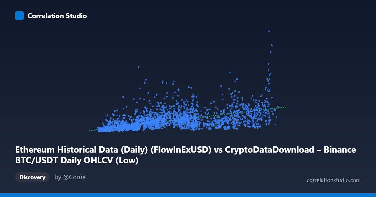
Ethereum Historical Data (Daily) (FlowInExUSD) vs CryptoDataDownload – Binance BTC/USDT Daily OHLCV (Low)
- Pearson correlation (r)
- 0.648
- Spearman correlation
- 0.8115
- p-value
- 0
- Sample size (n)
- 3191
- 95% confidence interval
- 0.6274 to 0.6676
- Granger causality
- Y → X
- Granger optimal lag
- 10
AI analysis
Analysis of the Relationship Between Two Metrics
Note on labeling: The axis descriptions appear crossed or mislabeled (the X-axis is described as an Ethereum flow metric, but its range and the Y-axis description reference BTC/USDT OHLCV data). For clarity, this analysis treats the variables purely as "X" and "Y" per the numeric data provided, since the substantive statistical relationship is what matters here.
1. What the Visualization Reveals
The scatterplot shows a positive, moderately strong association between X and Y: as X increases, Y tends to increase as well. However, the relationship is clearly not a simple straight line — Y's spread (stdev ≈ 613M, over 10x its own scale relative to X's stdev) suggests substantial heteroscedasticity, with the variance in Y growing considerably at higher X values. The data likely fans out into a cone or wedge shape typical of multiplicative/proportional relationships rather than additive linear ones.
2. Strength, Direction, and Statistical Confidence
The Pearson correlation (r = 0.648) indicates a moderate-to-strong positive linear relationship, with r² = 0.420 meaning X accounts for only about 42% of the variance in Y — leaving the majority (58%) unexplained by a linear model alone. The 95% CI [0.627, 0.668] is tight given the large sample (n=3,191), and the p-value of ~0 confirms this correlation is highly statistically significant and not due to chance. However, statistical significance here reflects the large sample size more than practical predictive strength — r² of 0.42 means X alone is a weak-to-moderate predictor of Y in isolation.
The Granger causality results are particularly noteworthy: Y Granger-causes X (F=2.67, p=0.003), while X does not Granger-cause Y (F=1.48, p=0.140). This suggests that past values of Y have predictive power for future values of X (at a 10-period lag), but not vice versa. This is a temporal precedence finding, not proof of causal mechanism — it implies Y's historical movements help forecast X's future movements more than the reverse.
3. Notable Patterns and Outliers
Several sample points show dramatic divergence from the fitted line — e.g., X≈35,440 paired with Y≈1.57B, X≈56,692 paired with Y≈1.79B, and X≈9,900 paired with Y≈588M — all substantially above what the linear model (y = 12,443.6x + 95.97M) would predict. These "spikes" in Y at moderate/low X values suggest occasional decoupling, possibly driven by episodic events (e.g., network congestion, exchange flow surges, or market shocks) unrelated to the baseline X-Y relationship. The note that Spearman's ρ exceeds Pearson's r is an important diagnostic — it indicates the rank-order relationship is stronger than the linear one, reinforcing that a monotonic non-linear model (log, power, or polynomial) would fit better, especially given Y's multi-order-of-magnitude range (14.4M to 6.92B).
4. Confounding Factors and Caveats
Both variables stem from cryptocurrency market/network data across an 8+ year span (2017–2026) covering multiple bull/bear cycles, halving events, and macro regime shifts (e.g., 2018 crash, 2020-21 bull run, 2022 collapse, subsequent recovery). Time itself is a likely lurking confounder — both series may be co-trending upward due to overall market growth, adoption, or inflationary price effects rather than a direct mechanical link between them. Additionally, since one series is described as a flow/volume metric and the other as a price-derived (OHLCV Low) metric, any shared dependence on overall market capitalization, trading activity, or volatility regime could inflate the observed correlation without genuine direct causation.
5. Actionable Insights
1. Refit with a non-linear model: Given the Spearman/Pearson divergence and Y's multi-order-of-magnitude spread, apply a log-log or log-linear transformation before regression — this will likely raise explained variance substantially. 2. Investigate lagged/Granger relationship further: Since Y leads X at a 10-period lag, build a vector autoregression (VAR) or lagged regression model using Y's history to predict X, and backtest this for practical forecasting value. 3. Control for time/trend: Detrend both series (e.g., via differencing or year-fixed effects) to test whether the correlation holds beyond shared market growth — this will clarify whether the r=0.648 reflects genuine covariation or a common time trend. 4. Examine outlier periods: Flag and investigate the dates behind the large positive residuals (e.g., Y spikes at low-moderate X) — these may correspond to specific market events worth excluding or modeling separately.
X dataset: CryptoDataDownload – Binance BTC/USDT Daily OHLCV
Y dataset: Ethereum Historical Data (Daily)
Part of experiment: Bitcoin - CryptoDataDownload – Binance BTC/USDT Daily OHLCV vs Ethereum Historical Data (Daily)