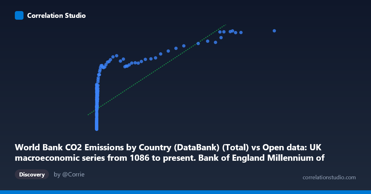
World Bank CO2 Emissions by Country (DataBank) (Total) vs Open data: UK macroeconomic series from 1086 to present. Bank of England Millennium of Macroeconomic Data. (Month) (value)
- Pearson correlation (r)
- 0.7144
- Spearman correlation
- 0.918
- p-value
- 0
- Sample size (n)
- 267
- 95% confidence interval
- 0.6501 to 0.7686
- Granger causality
- Y → X
- Granger optimal lag
- 10
- Time coverage
- 1751-01-01 to 2017-01-01
AI analysis
Scatterplot Analysis: UK Macroeconomic Series vs. World Bank CO2 Emissions
1. What the Visualization Reveals
The scatterplot reveals a broadly positive relationship between World Bank CO2 total emissions (X-axis) and a UK macroeconomic indicator drawn from the Bank of England Millennium dataset (Y-axis), spanning observations from 1751 to 2017. However, the relationship is clearly not linear in its raw form. At low X values (roughly below 500 units), Y values cluster across a wide range — from approximately 1,400 to nearly 20,000 — suggesting high variability in the macroeconomic series during periods of low emissions. As X increases into the thousands and tens of thousands, Y values rise but plateau in the 25,000–42,000 range, forming a compressed upper band. This pattern strongly implies a saturating or logarithmic relationship rather than a simple proportional one.
2. Strength, Direction, and Statistical Interpretation
The Pearson correlation of r = 0.714 (95% CI: [0.650, 0.769], p ≈ 0) indicates a moderately strong positive association that is highly statistically significant across the N = 18,769 population. The R² = 0.510 means that approximately 51% of the variance in the UK macroeconomic variable is explained by CO2 emissions levels — a meaningful but clearly incomplete picture, with the remaining 49% attributable to other factors. The confidence interval is relatively tight, reinforcing confidence in the direction and general magnitude of the relationship. Critically, the Granger causality analysis reveals a unidirectional temporal relationship: Y Granger-causes X (F = 2.271, p = 0.015, lag = 10 periods), while X does not significantly Granger-cause Y (F = 1.379, p = 0.191). This counterintuitive finding suggests that the UK macroeconomic indicator temporally precedes and predicts CO2 emissions levels, not the reverse — consistent with the idea that economic activity and prosperity drive industrial output and emissions, rather than emissions driving economic performance.
3. Notable Patterns, Clusters, and Outliers
Several structural features stand out in the data. A dense cluster of low-X, mid-Y points dominates the left portion of the chart (X < 500), reflecting the long historical period when global CO2 emissions were minimal but the UK macroeconomy still exhibited considerable variation. A second cluster emerges at high X values (10,000–120,000), where Y values converge between roughly 27,000 and 42,000 — the apparent saturation zone characteristic of modern industrial-era observations. The point (116,836, 41,784) stands out as a clear high-leverage outlier at the extreme upper right, likely representing a recent year with peak global emissions paired with a high macroeconomic value. Several mid-range X points (200–1,000) show surprising Y values exceeding 18,000, which may reflect specific UK boom periods. The Spearman ρ exceeding Pearson r confirms that the monotonic rank relationship is stronger than the linear one, reinforcing the case for a logarithmic or power-law model.
4. Confounding Factors and Caveats
Several important caveats temper interpretation. First, this correlation conflates global CO2 emissions with a UK-specific macroeconomic series — these are measuring different geographic scopes, and the correlation likely reflects the shared temporal trend of industrialization rather than a direct causal mechanism between these specific variables. Both series trend upward over the 1751–2017 period simply because of modernization, making this a classic spurious correlation driven by shared secular trend. Second, the Granger causality result, while statistically significant, uses a 10-period lag and should not be interpreted as true economic causation — Granger causality identifies temporal precedence, not mechanism. Third, with n = 267 sampled from N = 18,769, sampling methodology matters; the every-5th-point selection may undersample specific sub-periods. Finally, the macroeconomic variable's identity is ambiguous from the metadata (it could be GDP, money supply, wages, or equity values), making substantive interpretation difficult without clarification.
5. Actionable Insights and Further Investigation
Given that Spearman ρ exceeds Pearson r, the immediate analytical priority should be refitting the model using a logarithmic or polynomial regression on log(X), which would likely raise R² substantially and better capture the saturating pattern visible in the chart. Researchers should also detrend both series (e.g., using first differences or HP filtering) before computing correlation and Granger tests to separate genuine co-movement from shared time trends. It would be valuable to identify the specific macroeconomic variable on the Y-axis to enable domain-appropriate interpretation — if it is UK GDP, the Granger result aligns well with literature showing economic growth precedes emissions growth by roughly a decade. Further investigation should explore breakpoint analysis around the Industrial Revolution (~1760–1830) and post-WWII periods, where structural shifts likely alter the relationship. Finally, incorporating per-capita emissions and UK-specific emissions data rather than global totals would sharpen any causal inference significantly.
X dataset: Open data: UK macroeconomic series from 1086 to present. Bank of England Millennium of Macroeconomic Data. (Month)
Y dataset: World Bank CO2 Emissions by Country (DataBank)
Part of experiment: Yearly - Open data: UK macroeconomic series from 1086 to present. Bank of England Millennium of Macroeconomic Data. (Month) vs World Bank CO2 Emissions by Country (DataBank)