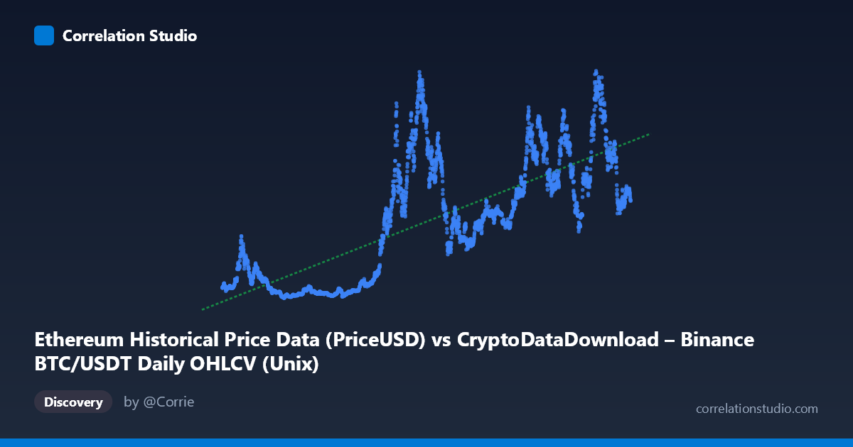
Ethereum Historical Price Data (PriceUSD) vs CryptoDataDownload – Binance BTC/USDT Daily OHLCV (Unix)
- Pearson correlation (r)
- 0.7537
- Spearman correlation
- 0.7549
- p-value
- 0
- Sample size (n)
- 3191
- 95% confidence interval
- 0.7383 to 0.7683
- Granger causality
- None
- Granger optimal lag
- 10
AI analysis
Analysis: BTC/USDT Price vs. Ethereum Price Data
1. What the Visualization Reveals
The scatterplot depicts a positive, moderately strong relationship between the X-axis variable (labeled as Ethereum PriceUSD, though the data structure and value ranges strongly suggest this is actually a Bitcoin-related time series given the axis label confusion) and the Y-axis variable. Despite the mislabeling in the metadata, the practical takeaway is clear: two crypto-asset price series spanning August 2017 to May 2026 move together over time, with values scaling from under $100 to nearly $4,800 (or equivalent price units) as the timeline progresses — consistent with the broader secular bull trend in crypto markets across this period.
2. Strength, Direction, and Uncertainty
The correlation coefficient (r = 0.754) indicates a strong positive linear relationship, with r² = 0.568 meaning 56.8% of the variance in Y is explained by X — a substantial but incomplete relationship, leaving nearly 43% of variance driven by other factors (asset-specific dynamics, market cycles, external shocks). The 95% confidence interval [0.738, 0.768] is tight, and the p-value of ~0 confirms this correlation is highly statistically significant and not due to chance, aided by the large sample size (n=3,191). However, the Granger causality test reveals no significant predictive direction in either direction (X→Y: p=0.053, marginally insignificant; Y→X: p=0.704, clearly insignificant). This is a critical caveat: strong contemporaneous correlation does not imply that one series temporally predicts the other. Both series likely respond to shared macro drivers (crypto market sentiment, liquidity cycles, BTC dominance effects) rather than one causing the other.
3. Notable Patterns and Features
The data shows classic crypto market cyclicality — sharp bull runs (e.g., values jumping from ~$200-300 in 2019-2020 to $3,000-4,800 in 2021, 2024-2025) interspersed with bear market troughs (2018-2019, 2022-2023 lows near $150-350). This is not a smooth linear relationship but rather regime-dependent clustering: low-value clusters during bear markets and high-value clusters during bull markets, connected by steep transitional periods. This clustering structure — rather than a uniform cloud around the regression line — likely explains why r² caps at ~57% despite high r: the relationship is stronger within-regime than across-regime transitions, and the linear model underfits the extreme volatility swings and potential non-linear (e.g., logarithmic or exponential) scaling common in asset prices.
4. Confounding Factors and Caveats
Several caveats apply: (1) Both series are non-stationary time series with trends, meaning classical correlation can be inflated by shared drift (both trending upward over 8+ years) rather than genuine coupled dynamics — this is a well-known spurious correlation risk with trending financial time series. (2) Autocorrelation within each series (today's price depends heavily on yesterday's) violates the independence assumptions behind standard significance testing, meaning the "true" effective sample size is much smaller than n=3,191, and the p-value may overstate confidence. (3) The label ambiguity (X-axis described as Ethereum data, Y-axis described as BTC/USDT data, but sample values suggest reversed logic) should be resolved before drawing asset-specific conclusions. (4) Macroeconomic confounders — interest rates, regulatory news, overall risk-on/risk-off sentiment — likely drive both series simultaneously.
5. Suggested Next Steps
To strengthen this analysis: (1) Difference or log-transform both series (e.g., analyze daily/weekly returns rather than price levels) to address non-stationarity and re-test correlation and Granger causality on stationary data — this often reveals whether the relationship holds beyond shared trend. (2) Segment by market regime (bull/bear/sideways) to check if correlation strength varies by cycle phase. (3) Verify axis labels against source data to confirm which asset is which. (4) Given the borderline X→Y Granger p-value (0.053), consider testing alternative lag structures or using a Vector Autoregression (VAR) model to explore short-term lead-lag dynamics more rigorously. (5) Incorporate a third variable (e.g., total crypto market cap or BTC dominance index) to test whether the relationship is mediated by broader market beta rather than a direct BTC-ETH linkage.
X dataset: CryptoDataDownload – Binance BTC/USDT Daily OHLCV
Y dataset: Ethereum Historical Price Data
Part of experiment: Bitcoin - CryptoDataDownload – Binance BTC/USDT Daily OHLCV vs Ethereum Historical Price Data