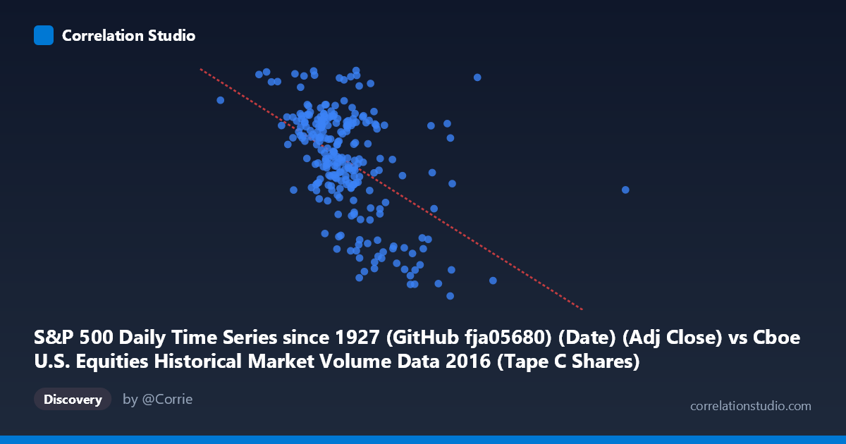
S&P 500 Daily Time Series since 1927 (GitHub fja05680) (Date) (Adj Close) vs Cboe U.S. Equities Historical Market Volume Data 2016 (Tape C Shares)

Pearson correlation (r): -0.5091
Spearman correlation: -0.5
p-value: 0
Sample size (n): 252
95% confidence interval: -0.5952 to -0.4114
Granger causality: None
Granger optimal lag: 4

AI analysis

Analysis: S&P 500 Price vs. Cboe Tape C Share Volume (2016)

Relationship Overview The scatterplot reveals a moderate negative relationship between S&P 500 adjusted closing prices (X-axis) and Cboe Tape C share volumes (Y-axis) across 252 trading days in 2016. As the S&P 500 index level increases, Tape C share volume tends to decline. This inverse pattern aligns with a well-documented market phenomenon: trading volume often contracts during calm, trending bull markets as uncertainty diminishes and the urgency to trade decreases. The linear regression equation (y = -1.8959E-06x + 2346.72) quantifies this, indicating that for every ~527 million point increase in the index, Tape C volume drops by approximately 1 share unit on the scale shown.

Correlation Strength and Statistical Robustness The Pearson correlation of r = -0.5091 reflects a moderate negative association, but the more meaningful figure is r² = 0.2592 — meaning S&P 500 price levels explain only about 26% of the variance in Tape C volume. The remaining 74% is driven by factors outside this model. The 95% confidence interval of [-0.5952, -0.4114] is reasonably tight and does not cross zero, and the p-value of effectively 0 confirms this relationship is highly statistically significant across the population of N = 3,622 observations. However, statistical significance should not be conflated with practical magnitude — the explained variance is modest. Critically, Granger causality tests yield no significant directional predictability in either direction (X→Y: F = 0.9458, p = 0.4381; Y→X: F = 1.4135, p = 0.2301), meaning that past S&P 500 prices do not reliably predict future Tape C volume, nor does volume predict future prices at the tested 4-period lag. The correlation is associative, not temporally predictive.

Notable Patterns and Outliers Several features stand out in the sample data. The bulk of observations cluster in the X range of approximately 107M–155M (index values), with Y values concentrated between roughly 2040–2200, forming a discernible downward-sloping core. However, there are notable outliers and dispersion at both extremes: points near x ≈ 99.8M show unusually high volume (~2265), while points near x ≈ 175M and x ≈ 315M (from the full range) correspond to markedly lower volumes (~1869–1893). The full X range extends dramatically to ~315M, suggesting the complete dataset contains high-index-level periods with substantially suppressed volume. There also appears to be heteroscedasticity — variance in volume is wider at lower index levels and compresses at higher levels — hinting that a simple linear model may not fully capture the relationship's shape.

Confounding Factors and Caveats Several important caveats apply. First, Tape C specifically covers NYSE Arca-listed securities, so this represents a subset of total market activity, not aggregate volume. Second, the S&P 500 index level is a composite price measure, not a direct driver of volume — it serves as a proxy for overall market conditions. Third, seasonal effects are likely embedded in 2016 data: volume is typically lower in summer months and higher in January and around major market events (e.g., Brexit in June 2016, U.S. election in November). Fourth, the relationship could be spurious or confounded by the secular upward drift in equity prices throughout 2016 coinciding with structural shifts in algorithmic and ETF trading volumes. The lack of Granger causality strongly suggests the correlation reflects shared dependence on underlying market regime variables rather than a direct causal link.

Actionable Insights and Further Investigation Practitioners should avoid using S&P 500 price levels alone to forecast Tape C volume — the 26% explained variance and absent Granger causality make this an unreliable predictive tool. More productive next steps would include: (1) incorporating VIX (volatility index) as a covariate, since fear/uncertainty is a stronger theoretical driver of volume than price level; (2) decomposing the time series seasonally to isolate structural volume patterns from market-regime effects; (3) testing non-linear models (e.g., polynomial or piecewise regression) given the apparent heteroscedasticity; (4) expanding to other Tape classifications (A and B) to assess whether this inverse relationship holds market-wide or is Tape C-specific; and (5) examining whether specific 2016 macro events (Brexit, Fed rate decisions, U.S. election) create identifiable regime breaks that distort the overall correlation.

X dataset: Cboe U.S. Equities Historical Market Volume Data 2016

Y dataset: S&P 500 Daily Time Series since 1927 (GitHub fja05680) (Date)

Part of experiment: Daily - Cboe U.S. Equities Historical Market Volume Data 2016 vs S&P 500 Daily Time Series since 1927 (GitHub fja05680) (Date)