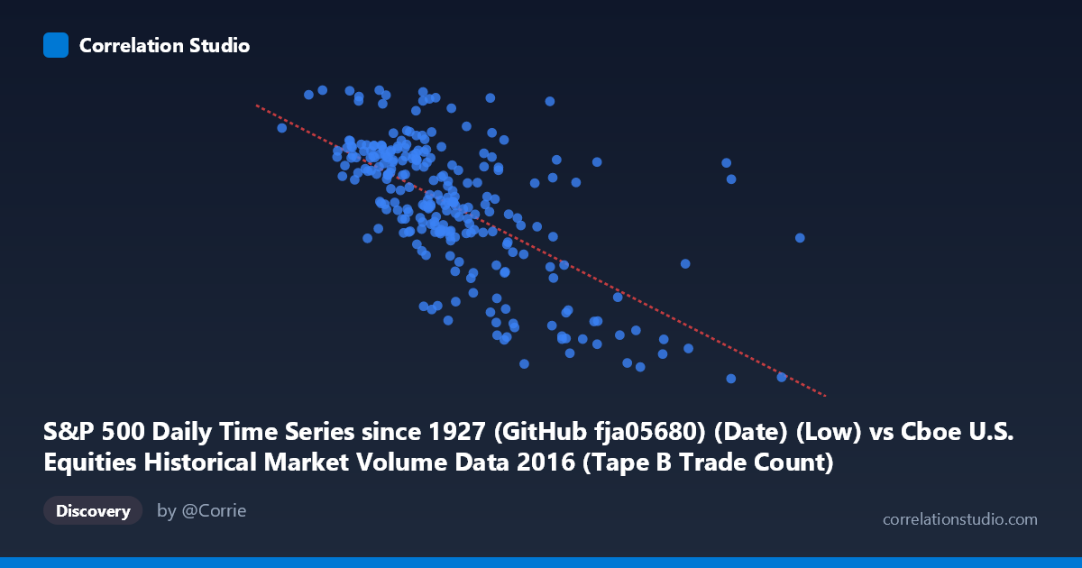
S&P 500 Daily Time Series since 1927 (GitHub fja05680) (Date) (Low) vs Cboe U.S. Equities Historical Market Volume Data 2016 (Tape B Trade Count)
- Pearson correlation (r)
- -0.6397
- Spearman correlation
- -0.6432
- p-value
- 0
- Sample size (n)
- 252
- 95% confidence interval
- -0.7074 to -0.5605
- Granger causality
- None
- Granger optimal lag
- 1
AI analysis
Analysis: S&P 500 Daily Low vs. Cboe Tape B Trade Count (2016)
Relationship Overview The scatterplot reveals a moderate negative relationship between the S&P 500 daily low price (X-axis) and the Cboe Tape B trade count (Y-axis) across 252 trading days in 2016. As the S&P 500 daily low increases — reflecting higher market price levels — the number of Tape B trades tends to decrease. The linear regression equation (y = −0.00071123x + 2310.85) quantifies this inverse slope, suggesting that for every 100,000-point increase in the daily low, trade count falls by roughly 71 units. Visually, the data points form a downward-sloping cloud concentrated in the X range of approximately 230,000–380,000, with a visible upper-left to lower-right trend, though with considerable scatter throughout.
Correlation Strength and Statistical Significance The Pearson correlation of r = −0.6397 indicates a moderate-to-strong negative association, and the R² of 0.4093 means that roughly 41% of the variance in Tape B trade counts is statistically explained by the S&P 500 daily low — a meaningful but far from complete explanation, leaving ~59% of variance attributable to other factors. The 95% confidence interval [−0.7074, −0.5605] is relatively tight and entirely negative, reinforcing confidence in the direction of the relationship. The p-value of effectively 0 (against N = 3,622) confirms this is not a chance finding. However, the Granger causality tests yield no significant predictive direction in either direction (X→Y: F = 0.51, p = 0.48; Y→X: F = 0.15, p = 0.70), meaning that despite the contemporaneous correlation, neither variable reliably predicts the other at the next time step. This is a critical distinction: the variables move together without one temporally leading the other.
Notable Patterns, Clusters, and Outliers The bulk of observations cluster between X values of ~230,000–370,000 and Y values of ~2,040–2,200, forming a relatively dense core. Several notable outliers stand out: points at very high X values (~558,190 and ~467,365) with low trade counts (~1,849 and ~1,873) lie in the lower-right extreme, potentially representing periods of high market prices with reduced trading activity. Conversely, one point near X ≈ 202,782 with Y ≈ 2,265 sits at the upper-left extreme — a low S&P price paired with high trade activity, consistent with early-2016 market turbulence. A point at (362,471, 2,254) also appears anomalously high in trade count for its price range. The scatter is heteroscedastic, appearing somewhat wider in the mid-range of X values, and there may be a slight non-linear (concave) curvature suggesting the relationship flattens at higher price levels.
Confounding Factors and Caveats Several important caveats apply. Most critically, this correlation likely reflects a shared temporal trend rather than a direct causal mechanism: in early 2016, the S&P 500 experienced a significant drawdown (low prices, high volatility, elevated trading activity), while the second half saw a recovery (higher prices, calmer markets, lower Tape-B volumes). This means the correlation may largely be capturing market regime changes — high-fear vs. low-fear periods — rather than a structural price-volume relationship. Additionally, Tape B specifically covers NYSE American (AMEX) and regional exchange stocks, which may not perfectly represent overall market sentiment. The note that the datasets originate from different sources (Cboe volume data merged with S&P 500 price data) introduces potential alignment or aggregation mismatches. Seasonality and macroeconomic events (e.g., Brexit in June 2016, U.S. election in November) could independently drive both variables simultaneously.
Actionable Insights and Further Investigation Given that ~59% of variance remains unexplained and Granger causality is absent, practitioners should avoid using S&P 500 price levels alone as a predictive signal for Tape B trade volume. Further investigation should include: (1) decomposing the time series to separate trend from cyclical components and re-testing correlation on detrended data to assess whether the relationship persists outside of the broad 2016 trend; (2) incorporating VIX (volatility index) as a covariate, since fear/volatility likely drives both lower prices and higher trade counts more directly; (3) examining Tape A and Tape C volumes comparatively to determine if this inverse pattern is exchange-specific or market-wide; and (4) extending the analysis beyond 2016 to test whether the observed correlation is stable across different market regimes or an artifact of this particular year's trajectory.
X dataset: Cboe U.S. Equities Historical Market Volume Data 2016
Y dataset: S&P 500 Daily Time Series since 1927 (GitHub fja05680) (Date)
Part of experiment: Daily - Cboe U.S. Equities Historical Market Volume Data 2016 vs S&P 500 Daily Time Series since 1927 (GitHub fja05680) (Date)