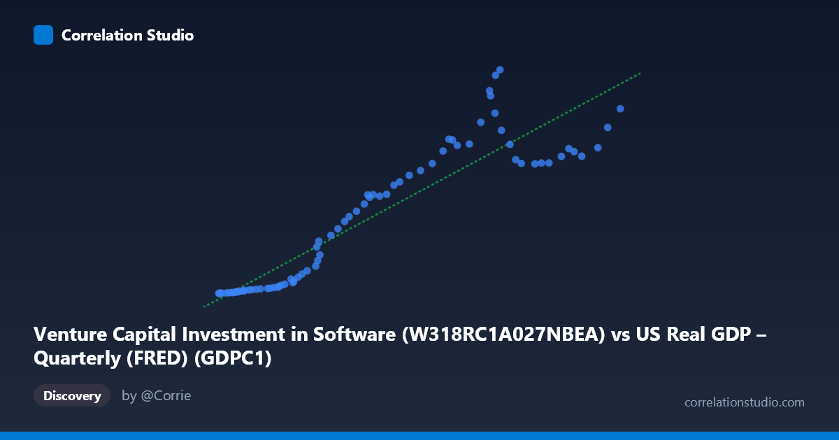
Venture Capital Investment in Software (W318RC1A027NBEA) vs US Real GDP – Quarterly (FRED) (GDPC1)
- Pearson correlation (r)
- 0.9219
- Spearman correlation
- 0.9558
- p-value
- 0
- Sample size (n)
- 78
- 95% confidence interval
- 0.8798 to 0.9496
- Granger causality
- None
- Granger optimal lag
- 10
- Time coverage
- 1947-01-01 to 2024-01-01
- Recomputed on refreshed data
- 2026-10-09 (r was 0.922)
AI analysis
Analysis: Venture Capital Software Investment vs. US Real GDP
Relationship Overview
The scatterplot reveals a strong positive relationship between Venture Capital Investment in Software and US Real GDP, with values spanning several decades (1947–2024). As real GDP increases from roughly $2,200B to $23,100B, software investment rises from near zero to over $466B. However, the relationship is not purely linear — the data exhibits a pronounced curve, particularly at lower GDP values (below ~$8,000B) where software investment remains extremely compressed, followed by an accelerating upswing at higher GDP levels. This shape strongly suggests an exponential or power-law relationship rather than the linear model fitted here.
Correlation Strength and Statistical Significance
The Pearson correlation of r = 0.922 indicates a very strong positive association, and the R² of 0.85 means that 85% of the variance in software investment is explained by real GDP — a remarkably high figure for macroeconomic data. The 95% confidence interval of [0.880, 0.950] is notably tight, reflecting the large sample (n = 78) and consistent directionality. The p-value of essentially zero confirms this relationship is not a statistical artifact. However, Granger causality yields no significant predictive direction in either direction (X→Y: F = 0.498, p = 0.883; Y→X: F = 0.435, p = 0.922), meaning that despite the strong contemporaneous correlation, neither variable reliably predicts the other temporally at the optimal 10-period lag. This is a critical distinction: the correlation reflects co-movement over time, not a causal mechanism that could be exploited for forecasting.
Notable Patterns, Clusters, and Outliers
The data clusters into two visually distinct regimes. The lower-left cluster (GDP < ~$8,000B, software investment < ~$125B) is densely packed with points hugging near-zero software values, corresponding to earlier decades when software was not yet a standalone investment category. The upper-right region shows far more dispersion, with software investment ranging from ~$200B to $466B across similar GDP levels (~$13,000–$23,000B), suggesting increasing variance in more recent years. A few points stand out: (16,843, 466.42) and (16,352, 412.27) appear notably high for their GDP levels, potentially representing peak investment years with above-trend tech spending, while several high-GDP observations ($20,000B) cluster around relatively modest software values (~$285–$385B), suggesting some deceleration or plateau in recent years.
Confounding Factors and Caveats
Several important caveats temper interpretation. First, both variables are non-stationary time series that trend upward over time, meaning their correlation may largely reflect shared temporal drift rather than a direct structural relationship — a classic spurious regression risk. Second, the linear model is a poor functional fit for what appears to be a nonlinear (likely exponential or logistic) relationship; the R² of 0.85 understates the model misspecification at the tails. Third, changes in accounting standards, BEA methodology, and the definition of "software investment" have evolved substantially over this period, potentially distorting comparability across decades. Finally, macroeconomic confounders — including interest rate cycles, the dot-com boom/bust, the 2008 financial crisis, and post-pandemic fiscal expansion — likely drive both variables simultaneously without implying direct linkage between them.
Actionable Insights and Further Investigation
Given the nonlinear visual pattern, the immediate priority should be re-fitting the model using a log-log or exponential specification, which would likely yield a better functional fit and more interpretable elasticity coefficients. Researchers should also difference or detrend both series before assessing correlation to test whether the relationship survives removal of shared temporal trends. Extending the Granger causality test across a range of shorter lags (1–5 periods) may uncover shorter-horizon predictive dynamics obscured at lag 10. It would also be valuable to control for confounders such as interest rates, total private fixed investment, or technology sector employment to isolate whether software investment carries independent explanatory power beyond what GDP alone captures. Finally, examining the residuals from the high-GDP cluster — particularly years where software investment appears to plateau despite rising GDP — could reveal structural breaks coinciding with market saturation, regulatory shifts, or post-pandemic normalization in tech spending.
X dataset: US Real GDP – Quarterly (FRED)
Y dataset: Venture Capital Investment in Software
Part of experiment: Yearly - US Real GDP – Quarterly (FRED) vs Venture Capital Investment in Software