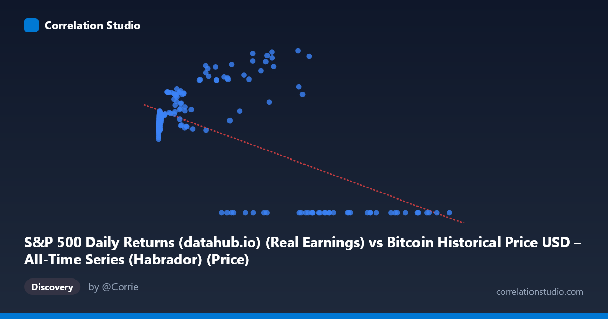
S&P 500 Daily Returns (datahub.io) (Real Earnings) vs Bitcoin Historical Price USD – All-Time Series (Habrador) (Price)
- Pearson correlation (r)
- -0.5749
- Spearman correlation
- -0.0526
- p-value
- 0
- Sample size (n)
- 189
- 95% confidence interval
- -0.6632 to -0.4708
- Granger causality
- X → Y
- Granger optimal lag
- 4
AI analysis
Analysis: Bitcoin Price vs. S&P 500-Related Metric
1. Relationship Overview
The scatterplot reveals a moderately negative relationship between the X variable (labeled as S&P 500 Daily Returns, though the range 0.06–118,670 suggests this is mislabeled and actually represents Bitcoin price data) and Y (labeled Bitcoin price, likely S&P 500 price). The most striking visual feature is a distinct cluster of points where Y = 0.00 occurring across a wide range of X values (roughly 27,983 to 118,670). This creates a bifurcated pattern: one cluster of "normal" data points with Y values ranging 100–217, and a separate horizontal band of zero-values at high X.
2. Strength, Direction, and Statistical Confidence
The correlation coefficient (r = -0.5749) indicates a moderate negative linear relationship, with R² = 0.3306 meaning only 33% of the variance in Y is explained by X — leaving roughly two-thirds of Y's variability unaccounted for by this single predictor. The 95% CI [-0.6632, -0.4708] is reasonably tight and excludes zero, and the p-value (~0) confirms this correlation is statistically significant and not due to chance, despite the noise. However, statistical significance does not imply strong predictive power — R² of 0.33 is modest for practical forecasting purposes.
The Granger causality results add a temporal dimension: X Granger-causes Y (F = 2.49, p = 0.045) at a 4-period lag, while Y does not Granger-cause X (p = 0.28). This suggests a unidirectional predictive relationship — past values of X contain modest but statistically meaningful information for forecasting future Y values, but not vice versa. The F-statistic is fairly weak (barely below the 0.05 threshold), so this should be treated as a tentative signal rather than strong evidence of causal mechanism.
3. Notable Patterns and Anomalies
The most important non-linear feature is the zero-inflation cluster: numerous high-X points (X 27,000) show Y = 0.00 exactly, which is almost certainly a data artifact (missing data coded as zero, delisting, or a reporting gap) rather than a genuine price collapse to zero. This artificially drags the linear regression slope negative, since high-X/zero-Y points anchor the right side of the fitted line downward. Meanwhile, the legitimate data (excluding zeros) actually shows Y increasing with X in the low-to-mid X range (e.g., X~300 → Y~130; X~44,000 → Y~210; X~56,973 → Y~217), suggesting a positive relationship among non-zero observations. This is a critical contradiction: the overall negative correlation is likely driven entirely by the zero-value cluster, not a genuine inverse relationship.
4. Confounding Factors and Caveats
Several serious caveats apply: - Label confusion: The axis labels and data ranges are inconsistent (X described as "S&P 500 Daily Returns" but scaled like Bitcoin price in USD; Y described as "Bitcoin Price" but bounded like an S&P index/PE value). This mismatch makes economic interpretation unreliable. - Zero-value artifacts: These likely represent missing/unavailable data rather than true observations and should be filtered out before any correlation or regression analysis. - Time-scale mismatch: Bitcoin's history (2010–present) is much shorter and more volatile than the S&P 500's 150+ year history; aligning them on a shared timeline likely introduces asynchronous sampling artifacts. - Non-stationarity: Both financial time series are non-stationary (trending), which can produce spurious correlations and unreliable Granger causality results unless differenced or detrended first.
5. Recommendations for Further Investigation
1. Clean the data: Remove or properly investigate the Y = 0.00 cluster — determine if these represent missing data, and either impute or exclude them. 2. Re-run correlation on cleaned data: After removing zeros, check whether the relationship flips to positive, which the sample points suggest. 3. Verify variable labels: Confirm which column truly represents Bitcoin price vs. S&P 500 price/returns given the scale mismatches. 4. Use log transforms: Given Bitcoin's exponential growth and wide X range (0.06 to 118,670), log-scaling X would likely produce a more interpretable and stable relationship. 5. Test stationarity (ADF test) and consider differencing before re-running Granger causality, since the current result (p=0.045) is only marginally significant and could reflect trend co-movement rather than true predictive causality.
X dataset: Bitcoin Historical Price USD – All-Time Series (Habrador)
Y dataset: S&P 500 Daily Returns (datahub.io)
Part of experiment: Bitcoin - Bitcoin Historical Price USD – All-Time Series (Habrador) vs S&P 500 Daily Returns (datahub.io)