World Bank CO2 Emissions by Country (DataBank) (Cement) vs Population, Total for United States (POPTOTUSA647NWDB) (POPTOTUSA647NWDB)
- Pearson correlation (r)
- 0.8995
- Spearman correlation
- 0.9902
- p-value
- 0
- Sample size (n)
- 61
- 95% confidence interval
- 0.8373 to 0.9387
- Granger causality
- None
- Granger optimal lag
- 10
- Time coverage
- 1960-01-01 to 2020-01-01
AI analysis
Scatterplot Analysis: U.S. Population vs. Cement CO₂ Emissions (1960–2020)
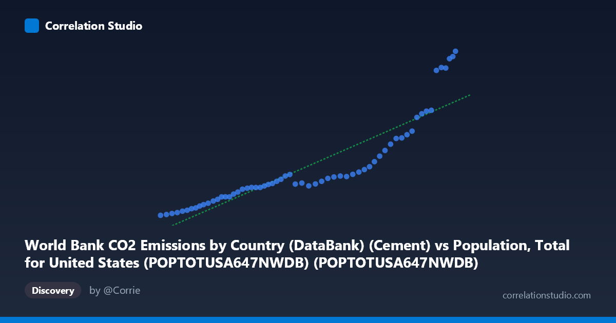
1. Overall Relationship The scatterplot reveals a strong positive association between total U.S. population and cement-related CO₂ emissions over the 1960–2020 period. As population grows from roughly 181 million to 332 million, cement emissions rise from approximately 247 to 2,609 units (likely thousand metric tons). The relationship is visibly non-linear — the data cluster tightly along a near-flat trajectory for lower population values (roughly 180–290 million), then curve sharply upward in the upper range (290–332 million), suggesting an accelerating or threshold-driven dynamic rather than a simple proportional relationship.
2. Correlation Strength and Statistical Interpretation The Pearson correlation of r = 0.900 indicates a very strong positive linear association, and r² = 0.809 means that approximately 80.9% of the variance in cement CO₂ emissions is statistically explained by population size alone. The 95% confidence interval for r [0.837, 0.939] is relatively narrow and does not approach zero, reinforcing that this is a robust, replicable relationship rather than a sample artifact. The p-value of effectively zero confirms it is highly unlikely to arise by chance. However, the Granger causality results are notably absent in both directions (X→Y: F = 0.748, p = 0.675; Y→X: F = 0.759, p = 0.665), meaning that neither variable temporally predicts the other beyond their shared trend — a critical caveat suggesting both are being driven by a third, underlying force (likely time/economic development) rather than one causing the other.
3. Patterns, Clusters, and Outliers The data divide visually into two distinct regimes. The lower-left cluster (population ~180–290 million, emissions ~247–1,100) spans roughly 1960–1990 and forms a dense, relatively flat band with modest emission growth per capita. The upper-right cluster (population ~290–332 million) shows dramatically steeper emission increases, consistent with post-1990s construction booms, infrastructure expansion, and urbanization acceleration. Several high-emission points near population values of 320–332 million (emissions exceeding 2,300–2,600 units) appear as potential outliers or leverage points that disproportionately anchor the regression slope. The linear regression equation y = 1.235×10⁻⁵x − 2,205.8 captures the overall trend but likely underfits the nonlinear upper-range behavior, as evidenced by the visible curve in the scatterplot.
4. Confounding Factors and Interpretive Caveats The most significant caveat is that both variables are time-indexed and trend upward together, making the correlation largely a reflection of shared temporal drift rather than a direct mechanistic link between population size and cement emissions. Economic growth, GDP expansion, construction cycles, infrastructure investment cycles, urbanization rates, and policy changes (e.g., highway acts, housing booms) are all plausible confounders that co-evolve with population. The sharp acceleration in the upper cluster may reflect the 1990s–2000s construction boom rather than population per se. Additionally, using a linear model on what appears to be a nonlinear (possibly exponential or piecewise) relationship risks systematic misestimation, and the Granger non-causality result strongly warns against any policy inference that population growth drives cement emissions or vice versa.
5. Actionable Insights and Further Investigation Several follow-up analyses are warranted: - Detrend both series (e.g., first-differencing or HP filter) before computing correlation to isolate genuine co-movement from shared time trends, which will almost certainly reduce the apparent r substantially. - Fit a nonlinear model (quadratic, log-log, or piecewise regression) to better characterize the accelerating upper-range behavior and test whether structural breaks exist around the 1990s. - Introduce per-capita cement emissions as the dependent variable to control for population scale directly, isolating whether emissions intensity is changing independently. - Add economic covariates (GDP, construction spending, housing starts) to a multivariate model to partition the variance more meaningfully. - Investigate the high-emission outlier years in the upper cluster to identify whether specific policy, economic, or methodological events explain the sharp departure from the lower-range trend.
X dataset: Population, Total for United States (POPTOTUSA647NWDB)
Y dataset: World Bank CO2 Emissions by Country (DataBank)
Part of experiment: Yearly - Population, Total for United States (POPTOTUSA647NWDB) vs World Bank CO2 Emissions by Country (DataBank)