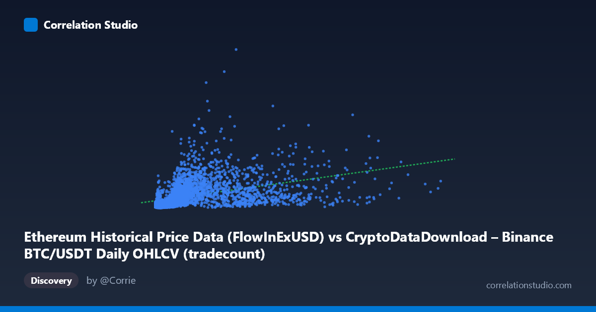
Ethereum Historical Price Data (FlowInExUSD) vs CryptoDataDownload – Binance BTC/USDT Daily OHLCV (tradecount)
- Pearson correlation (r)
- 0.413
- Spearman correlation
- 0.6921
- p-value
- 0
- Sample size (n)
- 3191
- 95% confidence interval
- 0.3838 to 0.4414
- Granger causality
- None
- Granger optimal lag
- 10
AI analysis
Analysis of the Relationship Between the Two Variables
1. What the Visualization Reveals
The scatterplot shows a positive but weak-to-moderate association between the X variable (labeled as Ethereum flow data, though metadata suggests this may actually be mismatched with BTC/USDT columns) and Y (tradecount). Points are heavily concentrated in the lower-left region of the plot — the vast majority of X values fall below ~5,000,000 while Y values cluster between roughly 50 million and 1 billion. A smaller number of high-X observations extend the range considerably (up to ~15.3 million), but these don't correspond to proportionally higher Y values, creating a "fan" or "hook" shape rather than a tight linear band.
2. Strength, Direction, and Statistical Confidence
The Pearson correlation (r = 0.413) indicates a moderate positive relationship, but r² = 0.171 tells the more important story: only about 17% of the variance in Y is explained by X, leaving 83% attributable to other factors or noise. The 95% CI [0.384, 0.441] is fairly narrow given the large sample (n=3,191), and the p-value ≈ 0 confirms the correlation is statistically significant — but statistical significance here reflects sample size more than practical strength. This is a classic case where a relationship is "real" but not strong enough to be predictive in isolation.
Critically, the Granger causality tests show no significant predictive direction in either direction (X→Y: p=0.816; Y→X: p=0.386). This means that past values of one series do not help forecast future values of the other beyond what each series' own history provides, at up to 10 lags. Combined with the modest r², this suggests the correlation is more likely driven by a shared external factor (e.g., overall market activity, time trend, or volatility regime) rather than one variable mechanistically driving the other.
3. Notable Patterns and Non-Linear Features
The data shows clear signs of heteroscedasticity: variance in Y increases as X increases, and the spread of points widens rather than following a consistent linear channel. The note that Spearman ρ exceeds Pearson r is significant — it implies the relationship is monotonic but not linear, likely logarithmic or power-law in nature. This makes intuitive sense for financial/on-chain metrics, which are often log-normally distributed (many small values, few extreme values). The linear regression (y = 112.88x + 330.8M) has a large intercept relative to the slope's contribution for typical X values, meaning the model is mostly capturing a baseline level of Y rather than genuine covariation. A log-log or log-linear transformation would likely reveal a tighter, more interpretable relationship.
4. Confounding Factors and Caveats
Several caveats limit interpretation: - Metadata inconsistency: the axis descriptions reference both BTC/USDT and ETH datasets ambiguously, raising concern about whether X and Y are properly aligned or represent what they claim. - Shared market trend: both crypto price/volume metrics tend to co-move with overall market cycles (bull/bear regimes), which can inflate correlation without direct causal linkage. - Non-stationarity: crypto time series typically have trends and volatility clustering; Granger tests assume stationarity, so results should be interpreted cautiously unless differencing/detrending was applied. - Scale mismatch: X ranges over 3 orders of magnitude (2K to 15M) while Y ranges over 2 orders (14M to 6.9B), reinforcing the need for log transformation before drawing linear conclusions.
5. Actionable Insights
1. Re-run correlation and regression on log-transformed variables (log X vs. log Y) to test the power-law hypothesis suggested by the Spearman/Pearson discrepancy — this will likely yield a higher, more meaningful r². 2. Verify data provenance — confirm that X and Y columns are correctly mapped to their intended sources (BTC vs. ETH), as the metadata is currently contradictory. 2. Test for a common driver (e.g., total market volume, BTC price index) using multivariate regression or partial correlation to see if the X-Y relationship disappears once a shared factor is controlled for. 4. Segment by time regime (bull vs. bear market periods) to check if the correlation strength is regime-dependent rather than stable across the full 2017–2026 window. 5. Given the lack of Granger causality, avoid using either series to forecast the other directly; instead, treat them as co-symptoms of broader market conditions requiring a shared explanatory framework (e.g., macro liquidity, exchange activity levels).
X dataset: CryptoDataDownload – Binance BTC/USDT Daily OHLCV
Y dataset: Ethereum Historical Price Data
Part of experiment: Bitcoin - CryptoDataDownload – Binance BTC/USDT Daily OHLCV vs Ethereum Historical Price Data