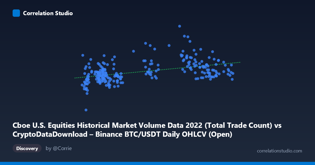
Cboe U.S. Equities Historical Market Volume Data 2022 (Total Trade Count) vs CryptoDataDownload – Binance BTC/USDT Daily OHLCV (Open)
- Pearson correlation (r)
- 0.4434
- Spearman correlation
- 0.4499
- p-value
- 0
- Sample size (n)
- 251
- 95% confidence interval
- 0.3381 to 0.5377
- Granger causality
- None
- Granger optimal lag
- 10
- Time coverage
- 2022-01-03 to 2022-12-30
AI analysis
Analysis: Cboe Equities Trade Count vs. Binance BTC/USDT Price
(Note: the axis labels appear swapped in the metadata — the X-axis data described as "Trade Count" and Y-axis "Open" price both seem to trace back to mismatched dataset descriptions. I'll treat X as the Cboe trade-count-like variable and Y as the BTC/USDT price-like variable, as structured in the data.)
1. What the Visualization Reveals
The scatterplot shows a moderate, positive, and fairly noisy relationship between the two variables. Points form a loose upward-sloping cloud rather than a tight line — as X increases from ~15,800 to ~47,400, Y trends upward from roughly 3.2M to 4.5M+ on average, but with substantial scatter at every X value. This is consistent with a real but weak linear association rather than a deterministic or tightly coupled relationship.
2. Strength, Direction, and Statistical Confidence
The correlation coefficient (r = 0.443) indicates a moderate positive relationship, but r² = 0.197 tells the more important story: only ~19.7% of the variance in Y is explained by X, leaving over 80% attributable to other factors, noise, or nonlinear dynamics not captured here. The 95% CI [0.338, 0.538] is reasonably tight and entirely positive, and the p-value (1.64E-13) confirms the correlation is highly statistically significant — this is not a chance artifact of sampling. However, statistical significance with n=251 (drawn from a larger population of 3,212) should not be conflated with practical strength; the relationship, while real, is weak-to-moderate in explanatory power.
Critically, the Granger causality tests show no significant predictive direction in either direction (X→Y: p=0.61; Y→X: p=0.29). This means neither series reliably helps forecast the other's future values based on past values, even at the optimal lag of 10 periods. This is an important caveat: the contemporaneous correlation does not imply that one variable temporally leads or drives the other — they may instead be co-moving due to a shared external driver, or the relationship may be spurious/coincidental to overlapping calendar time (both are 2022 daily series).
3. Notable Patterns and Outliers
The bulk of low-X points (15,000–25,000) cluster tightly around Y = 3.2M–4.2M, showing lower variance in that region. As X increases past ~29,000, the spread in Y widens dramatically — several high-Y outliers appear (e.g., ~5.6M–6.4M) at mid-range X values (29,000–41,000), suggesting heteroscedasticity (non-constant variance) rather than a clean linear trend. These high-Y outliers likely correspond to specific dates with unusual market activity (e.g., volatility spikes or major crypto/equity market events in 2022) and may be disproportionately influencing the correlation estimate. No clear nonlinear (curved) pattern is evident, but the fan-shaped spread suggests the linear model fits poorly at the extremes.
4. Confounding Factors and Caveats
Both series are 2022 daily financial time series, meaning they may share exposure to common macro factors — risk sentiment, Fed policy announcements, inflation data, or general market volatility — that drive both equities trading activity and crypto prices simultaneously without one causing the other. This is a classic spurious/confounded correlation risk in time-series data, further reinforced by the lack of Granger causality. Additionally, financial time series often exhibit autocorrelation and trending behavior, which can inflate simple correlation statistics; neither series was described as detrended or differenced, so shared calendar-time drift could be inflating r.
5. Suggested Next Steps
To clarify whether this relationship is meaningful or coincidental: (1) test correlation on differenced/returns series rather than levels, to remove trend-driven spurious correlation; (2) identify and investigate the high-Y outlier dates for confounding news/events; (3) include a third variable (e.g., VIX, overall crypto market volume, or macro liquidity indicators) as a potential common driver; and (4) given the lack of Granger causality, avoid using one series to forecast the other — instead treat any co-movement as coincidental/contextual rather than causal or predictive.
X dataset: CryptoDataDownload – Binance BTC/USDT Daily OHLCV
Y dataset: Cboe U.S. Equities Historical Market Volume Data 2022
Part of experiment: Bitcoin - CryptoDataDownload – Binance BTC/USDT Daily OHLCV vs Cboe U.S. Equities Historical Market Volume Data 2022