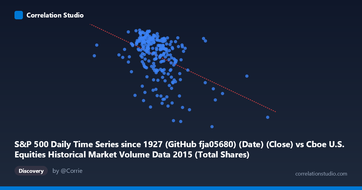
S&P 500 Daily Time Series since 1927 (GitHub fja05680) (Date) (Close) vs Cboe U.S. Equities Historical Market Volume Data 2015 (Total Shares)

Pearson correlation (r): -0.4486
Spearman correlation: -0.4142
p-value: 0
Sample size (n): 252
95% confidence interval: -0.5421 to -0.3441
Granger causality: X → Y
Granger optimal lag: 5

AI analysis

S&P 500 Close Price vs. Total Market Shares Traded (2015)

Relationship Overview The scatterplot reveals a negative relationship between the S&P 500 daily closing price (X-axis) and total U.S. equity shares traded (Y-axis) across 2015. As the index closed at higher levels, total share volume tended to be lower, and conversely, periods of lower closing prices corresponded with elevated trading volumes. This inverse pattern aligns with well-established market dynamics where volatility and fear-driven selling episodes drive both price declines and volume spikes simultaneously.

Correlation Strength and Statistical Significance The Pearson correlation of r = -0.4486 indicates a moderate negative association, but the coefficient of determination tells a more sobering story: R² = 0.2012, meaning the S&P 500 close price explains only about 20% of the variance in total shares traded. The remaining 80% is attributable to other factors entirely. The 95% confidence interval of [-0.5421, -0.3441] is entirely negative and comfortably excludes zero, and the p-value of 7.04×10⁻¹⁴ confirms this relationship is highly unlikely to be a chance finding in a sample of n=252 from a population of N=3,302. Critically, the Granger causality analysis supports a unidirectional temporal relationship: X Granger-causes Y at a 5-period lag (F=2.34, p=0.0425), while Y does not Granger-cause X (F=0.37, p=0.87). This suggests that S&P 500 price levels have modest but statistically meaningful predictive power over subsequent share volumes, roughly one trading week later, though this should not be mistaken for true structural causation.

Notable Patterns, Clusters, and Outliers Several features stand out in the data. The bulk of observations cluster between approximately 460M–580M on the X-axis and 2,040–2,130 on the Y-axis, representing the "normal" trading environment of mid-2015. A distinct lower-right cluster is absent, while a clear lower-left region (index values ~600M–850M, share prices ~1,867–1,990) captures the notable August–September 2015 market correction, where extreme volume accompanied sharp price declines — the point at (808M, 1,867) is a prominent outlier likely corresponding to the August 24th "flash crash" episode. Similarly, several high-volume, low-price points around (648M, 1,882) and (657M, 1,920) reinforce the correction cluster. These outliers exert meaningful leverage on the regression slope and likely inflate the correlation magnitude.

Confounding Factors and Caveats Several important caveats apply. First, the August 2015 correction is a confounding structural break — it simultaneously drove prices down and volume up, creating a natural negative correlation that may not persist in calmer regimes. Second, secular trends in both series (index gradually appreciating over the year while volume drifts) could produce spurious correlation even without a mechanistic link. Third, the linear model (y = -2.525×10⁻⁷x + 2,194.35) may be misspecified: the relationship likely has heteroskedastic variance, with volume dispersion widening at lower price levels, suggesting a non-linear or regime-dependent model might fit better. Fourth, Granger causality does not imply economic causation — the 5-lag predictive signal may simply reflect autocorrelated volatility clustering rather than any direct price-to-volume mechanism.

Actionable Insights and Further Investigation Practitioners should explore volatility regime segmentation — splitting the data into high-VIX and low-VIX periods to test whether the correlation is primarily driven by stress episodes or holds broadly. Substituting returns or log-price changes for closing levels would remove the trend component and test whether day-to-day price movements (not levels) predict volume more cleanly. Given the Granger result, a 5-day lagged regression model deserves formal testing as a potential short-term volume forecasting tool. Additionally, incorporating options market data or VIX levels as covariates would help isolate whether price levels per se drive volume, or whether both are jointly determined by an underlying volatility factor. Finally, extending the analysis to multiple years would reveal whether 2015's correction-dominated dynamic is representative or anomalous.

X dataset: Cboe U.S. Equities Historical Market Volume Data 2015

Y dataset: S&P 500 Daily Time Series since 1927 (GitHub fja05680) (Date)

Part of experiment: Daily - Cboe U.S. Equities Historical Market Volume Data 2015 vs S&P 500 Daily Time Series since 1927 (GitHub fja05680) (Date)