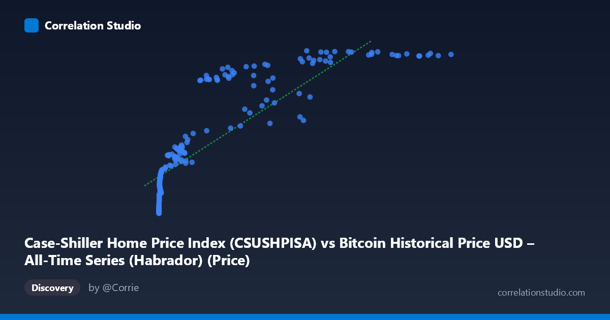
Case-Shiller Home Price Index (CSUSHPISA) vs Bitcoin Historical Price USD – All-Time Series (Habrador) (Price)
- Pearson correlation (r)
- 0.857
- Spearman correlation
- 0.97
- p-value
- 0
- Sample size (n)
- 192
- 95% confidence interval
- 0.8142 to 0.8905
- Granger causality
- None
- Granger optimal lag
- 2
- Time coverage
- 2010-08-01 to 2026-07-01
- Recomputed on refreshed data
- 2026-10-24 (r was 0.8512)
AI analysis
Analysis: Bitcoin Price vs. Case-Shiller Home Price Index
1. What the Visualization Reveals
The scatterplot shows a strong positive association between Bitcoin's historical USD price and the Case-Shiller Home Price Index (CSUSHPISA), but the relationship is clearly non-linear. At low Bitcoin values (under ~$1,000), the Case-Shiller Index clusters tightly in the 137–190 range. As Bitcoin's price climbs into the tens of thousands, the index rises into the 250–330 range, but the rate of increase flattens at the high end — a classic logarithmic or saturating curve rather than a straight line. This is unsurprising given Bitcoin's price spans nearly six orders of magnitude (0.06 to 118,670), while the index only ranges from 136 to 332.
2. Strength, Direction, and Uncertainty
The Pearson correlation (r = 0.849, r² = 0.721) indicates a strong positive linear relationship, with about 72% of the variance in one variable statistically explained by the other. The 95% CI [0.804, 0.885] is tight and does not cross zero, and the p-value is effectively 0, meaning this correlation is highly unlikely to be a sampling artifact. However, correlation here should not be read as causation — the Granger causality tests explicitly show no significant predictive relationship in either direction (X→Y: p=0.534; Y→X: p=0.539). This means neither variable's past values meaningfully help forecast the other's future values once autocorrelation is accounted for. The strong r is likely driven by both series independently trending upward over the same 2010–2026 period, not by one causing or leading the other.
3. Notable Patterns and Outliers
- Log-linear pattern: Since Spearman ρ likely exceeds Pearson r (per the note), rank-order correlation fits better than raw linear correlation — a log-transform of X would likely straighten the relationship substantially. - Dense low-end cluster: Many points sit at very small Bitcoin values (single digits to low hundreds) corresponding to the 2010–2013 era, all compressed near Y≈137–190. - Ceiling effect at high X: Once Bitcoin exceeds ~$60,000, the index plateaus near 320–332, suggesting diminishing marginal association — the index has real-world upper bounds (housing prices) that Bitcoin's speculative price does not share. - Some noisy scatter mid-range: Points like (45,092.81, 245.42) and (56,973.18, 281.53) show non-monotonic wobble, likely reflecting Bitcoin's volatility (crashes/bull runs) not mirrored by the comparatively stable housing index.
4. Confounding Factors and Caveats
This is a textbook case of spurious correlation via shared time trend. Both Bitcoin price and U.S. home prices have risen substantially since 2010, driven by entirely different macro forces: Bitcoin by adoption/speculation cycles, halvings, and crypto-specific sentiment; the Case-Shiller Index by mortgage rates, housing supply, wage growth, and monetary policy (especially post-2020 stimulus). Common confounders include general USD inflation, near-zero interest rate eras (2010–2021), and post-pandemic asset price inflation, which could lift both series simultaneously without any direct link. Additionally, sampling every 3rd point and the uneven time distribution (heavy weighting toward Bitcoin's low-price early years) may distort the apparent linear fit.
5. Suggestions for Further Investigation
- Detrend both series (e.g., using year-over-year % change or differencing) before correlating — this tests whether short-term movements co-vary, stripping out the shared long-term drift. - Log-transform Bitcoin price and re-run linear regression/correlation, given the non-linear shape already evident. - Control for a common macro variable (CPI, M2 money supply, Fed funds rate) via partial correlation to see if the Bitcoin–housing link survives. - Given the null Granger causality result, avoid using one series to forecast the other; instead treat this as two assets independently benefiting from the same low-rate, high-liquidity macro environment rather than a tradeable causal relationship.
X dataset: Bitcoin Historical Price USD – All-Time Series (Habrador)
Y dataset: Case-Shiller Home Price Index
Part of experiment: Bitcoin - Bitcoin Historical Price USD – All-Time Series (Habrador) vs Case-Shiller Home Price Index