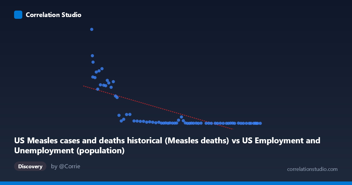
US Measles cases and deaths historical (Measles deaths) vs US Employment and Unemployment (population)
- Pearson correlation (r)
- -0.7317
- Spearman correlation
- -0.9209
- p-value
- 0
- Sample size (n)
- 74
- 95% confidence interval
- -0.8226 to -0.6042
- Granger causality
- None
- Granger optimal lag
- 10
- Time coverage
- 1949-01-01 to 2022-01-01
- Recomputed on refreshed data
- 2026-10-17 (r was -0.7317)
AI analysis
Analysis: US Measles Deaths vs. Population (1949–2022)
1. What the Visualization Reveals
The scatterplot displays a strong negative relationship between US Measles deaths (X-axis) and US population figures (Y-axis) over roughly seven decades. The data clearly clusters into two distinct behavioral zones: a high-X/high-Y region where measles deaths are numerous and population values are elevated, and a dense low-X/near-zero-Y cluster where deaths approach zero and population readings correspondingly collapse toward the baseline. This visual pattern reflects the dramatic historical decline in measles mortality following the introduction of the measles vaccine in 1963 and the subsequent expansion of immunization programs through the 1970s and beyond.
2. Correlation Strength, Direction, and Causal Framing
The Pearson correlation of r = -0.7317 indicates a strong negative association, meaning that as measles deaths increased historically, the population metric (as defined in this dataset) also increased — and as deaths fell, so did that metric. The coefficient of determination r² = 0.5353 tells us that approximately 53.5% of the variance in the Y variable is explained by X, which is a meaningful but incomplete explanatory share — nearly half the variance remains unaccounted for by this linear relationship alone. The 95% confidence interval of [-0.8226, -0.6042] is relatively tight and entirely negative, confirming the direction of the relationship with reasonable precision. The p-value of 1.319×10⁻¹³ is extraordinarily small, making it statistically implausible that this correlation arose by chance given the sample size of n=74.
However, the Granger causality tests are non-significant in both directions (X→Y: F=1.19, p=0.324; Y→X: F=1.63, p=0.131), meaning neither variable demonstrably predicts the other temporally at the optimal 10-period lag. This is a critical finding: despite the strong static correlation, there is no detectable temporal predictive signal — neither variable "leads" the other in a forecasting sense. This strongly implies the correlation reflects a shared common driver (time itself, or the historical arc of medical and public health progress) rather than any direct mechanistic link between measles deaths and the population metric as defined here.
3. Notable Patterns, Clusters, and Outliers
Several features stand out visually: - A high-leverage cluster in the lower-left (low X, low Y) represents recent decades where measles deaths are near zero and the Y metric correspondingly approaches zero — these points dominate the regression and compress variance. - A scattered upper-left arc of points (X: 104,000–130,000; Y: 260–949) represents earlier decades with high measles mortality and high population metric values. The point (103,994; 949) is a notable extreme outlier at the upper boundary of both distributions. - The relationship appears non-linear — the Spearman ρ exceeding Pearson r confirms this. A logarithmic or polynomial curve would likely fit substantially better than the linear model, capturing the steep drop in Y as X declines from peak values and the subsequent floor effect near zero. - The mid-range of X (roughly 130,000–170,000) shows high scatter in Y, suggesting a transitional period where both variables were declining but not in lockstep.
4. Confounding Factors and Caveats
This correlation is a textbook example of shared temporal trend confounding. Both measles deaths and this population metric declined over the same historical period for reasons driven by broader societal and medical forces — vaccination programs, improved healthcare infrastructure, public health policy, and rising living standards — rather than any direct causal link between the two specific variables. The dataset labeling itself raises concerns: the X-axis column is drawn from an employment/unemployment dataset labeled as "Measles deaths," and the Y-axis population column is drawn from a measles dataset — this cross-dataset pairing warrants careful verification that the columns are correctly matched and meaningfully comparable. Additionally, annual aggregation smooths within-year variation, and the 86-year time span means early data quality may differ substantially from modern reporting standards.
5. Actionable Insights and Further Investigation
- Do not interpret this as causal: the absence of Granger causality, combined with the obvious shared-trend structure, means this correlation should not inform policy decisions linking these two variables directly. - Fit a non-linear model (logarithmic or segmented regression) to better capture the evident curve in the scatterplot and improve on the 53.5% variance explained. - Investigate the pre/post-vaccine discontinuity explicitly by testing a structural break around 1963–1968; a piecewise regression may reveal that the relationship changes character entirely across that threshold. - Detrend both series before re-running correlation and Granger tests to remove the shared time trend and assess whether any residual relationship persists — this would provide a far more honest test of association. - Verify dataset column alignment: the cross-dataset column sourcing is unusual and should be confirmed to ensure the X and Y variables are what they are labeled to be before drawing any substantive conclusions.
X dataset: US Employment and Unemployment
Y dataset: US Measles cases and deaths historical
Part of experiment: Yearly - US Employment and Unemployment vs US Measles cases and deaths historical