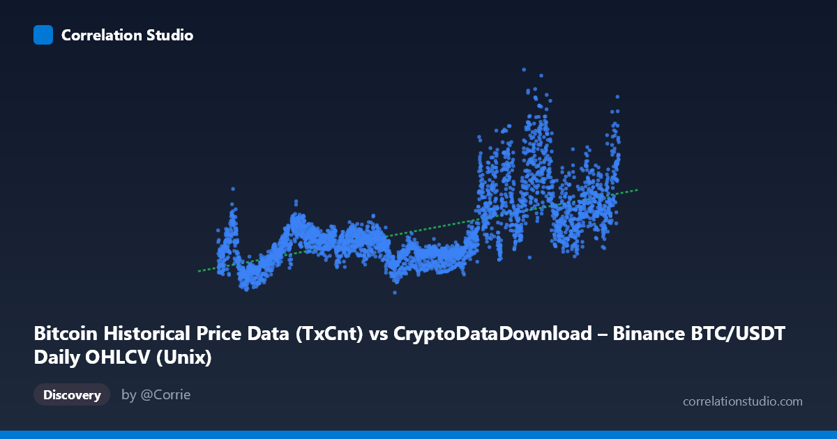
Bitcoin Historical Price Data (TxCnt) vs CryptoDataDownload – Binance BTC/USDT Daily OHLCV (Unix)
- Pearson correlation (r)
- 0.6143
- Spearman correlation
- 0.6107
- p-value
- 0
- Sample size (n)
- 3191
- 95% confidence interval
- 0.5922 to 0.6355
- Granger causality
- None
- Granger optimal lag
- 10
- Time coverage
- 2017-08-17 to 2026-05-20
AI analysis
Analysis: Bitcoin Time-Series Metric Correlation
1. What the Visualization Shows
Both the X and Y axes here are effectively time-indexed Bitcoin-related metrics (X is a timestamp-labeled column, Y is a Unix-timestamp-labeled column from OHLCV data), spanning August 2017 through mid-2026. Given the axis ranges, this scatterplot is essentially tracking how a Bitcoin-derived value trends over the calendar timeline. The scatter shows a broad, upward-sloping cloud of points — a general rise in Y-values as X (time) progresses — but with substantial vertical dispersion at any given point along the X-axis, indicating high volatility or noise layered on top of the trend.
2. Strength and Direction of the Relationship
The correlation coefficient (r = 0.614) indicates a moderate positive relationship. Squaring this, r² = 0.377, means only about 37.7% of the variance in Y is explained by X — the majority (62%) of Y's variability comes from other factors not captured by this simple linear relationship with time/X. The 95% confidence interval [0.592, 0.636] is tight and does not cross zero, and the p-value of effectively 0 confirms this correlation is highly statistically significant and not a product of chance, especially given the large sample (n=3,191). However, statistical significance should not be conflated with practical predictive strength — a moderate r² leaves considerable room for error in any forecasting application.
Critically, the Granger causality tests show no significant predictive direction in either direction (X→Y: p=0.171; Y→X: p=0.522). This is an important nuance: despite the contemporaneous correlation, neither variable's past values reliably help forecast the other's future values at the tested lag (10 periods). This suggests the correlation is likely driven by a shared underlying trend (e.g., both series reflecting long-term Bitcoin market growth or the passage of time itself) rather than one metric causally leading the other.
3. Notable Patterns and Features
The sampled data points reveal a clear cyclical, non-linear structure consistent with Bitcoin's known boom-bust cycles rather than a clean linear trend: - Early period (2017-2018): Y-values cluster in the 130,000–280,000 range - Mid period (2019-2021): increased volatility, values ranging widely from ~180,000 to over 400,000 - Later period (2023-2026): notably higher values, frequently exceeding 400,000–700,000, with a max of 928,131
This pattern suggests multiple regime shifts or bull/bear cycles superimposed on a general upward drift, rather than a smooth linear relationship. The linear R² of 0.377 likely understates the relationship's complexity — a piecewise or log-transformed model, or one incorporating cyclical/seasonal components, would likely fit much better than the straight line implied by y = 9.68e-07x − 1.24e6.
4. Confounding Factors and Caveats
Several caveats apply: - Spurious time-trend correlation: Since X appears to encode time (or a time-correlated variable) and Y is a price/volume-adjacent metric, both may simply be trending upward due to Bitcoin's overall market maturation and adoption — a classic case of two non-stationary time series appearing correlated without direct causal linkage. - Non-stationarity: Bitcoin price/volume data is well-documented as non-stationary (trending, heteroskedastic). Standard correlation and even Granger causality tests assume some degree of stationarity; results here should be interpreted cautiously without differencing or detrending the series first. - Regime dependency: Correlation strength likely varies dramatically across bull markets, crashes, and consolidation periods — a single global r may mask periods of much stronger or weaker association. - Data structure ambiguity: The unusual axis labels (X described as a price data column, Y described as a Unix timestamp column) suggest possible metadata/column mismatches — this should be verified before drawing strong conclusions.
5. Suggested Further Investigation
1. Detrend or difference both series (e.g., use daily returns/changes rather than levels) and re-run correlation and Granger tests — this will reveal whether the relationship holds beyond a shared time trend. 2. Segment by market regime (bull/bear/sideways) to see if r² is substantially higher within specific periods. 3. Test non-linear/log models given the cyclical, heteroskedastic pattern — a log-log or polynomial fit may explain more variance than the current linear model. 4. Verify data provenance — clarify what X and Y actually represent (the column descriptions seem inconsistent with typical axis conventions) to ensure the analysis is interpreting the right variables. 5. Given the lack of Granger causality, avoid using one series to predict the other in a trading or forecasting context; instead, treat the correlation as descriptive of a shared macro trend rather than an exploitable predictive signal.
X dataset: CryptoDataDownload – Binance BTC/USDT Daily OHLCV
Y dataset: Bitcoin Historical Price Data
Part of experiment: Bitcoin - CryptoDataDownload – Binance BTC/USDT Daily OHLCV vs Bitcoin Historical Price Data