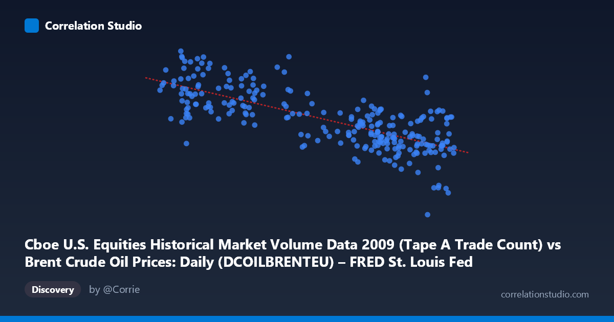
Cboe U.S. Equities Historical Market Volume Data 2009 (Tape A Trade Count) vs Brent Crude Oil Prices: Daily (DCOILBRENTEU) – FRED St. Louis Fed (DCOILBRENTEU)
- Pearson correlation (r)
- -0.7366
- Spearman correlation
- -0.719
- p-value
- 0
- Sample size (n)
- 252
- 95% confidence interval
- -0.7884 to -0.6744
- Granger causality
- None
- Granger optimal lag
- 10
AI analysis
Analysis: Brent Crude Oil Price vs. U.S. Equity Trade Count (2009)
Relationship Overview The scatterplot reveals a moderate-to-strong negative relationship between Cboe U.S. equity trade counts (Tape A) and Brent crude oil prices in 2009. As daily trade volume activity increases, crude oil prices tend to be lower, and conversely, lower trading activity coincides with higher oil prices. The linear regression equation (y = -23,226.1x + 3,063,290) quantifies this inverse slope: each additional unit increase in trade count is associated with a decrease of approximately 23,226 units in the Y variable (trade count in oil dataset context). The negative slope is visually apparent across the bulk of the data cloud, though with considerable scatter around the trend line.
Correlation Strength and Statistical Framing The Pearson correlation of r = -0.7366 indicates a meaningful negative association, and the R² of 0.5426 means that roughly 54.3% of the variance in Y is explained by X — a substantial but incomplete explanatory relationship, leaving ~46% attributable to other factors. The 95% confidence interval of [-0.7884, -0.6744] is relatively tight and entirely negative, reinforcing confidence in the direction of the relationship. The p-value of effectively zero, drawn from a population of N = 3,232 with a paired sample of n = 252, confirms this is highly statistically significant and not a chance artifact. However, despite the strong correlation, Granger causality tests find no significant predictive directionality in either direction (X→Y: F = 1.51, p = 0.137; Y→X: F = 1.20, p = 0.289) even at the optimal 10-period lag. This is a critical caveat: the variables move together, but neither demonstrably leads the other temporally, suggesting the relationship is associative rather than predictive in a time-series sense.
Notable Patterns, Clusters, and Outliers Several features stand out visually. The data cloud shows a reasonably consistent negative trend but with heteroscedastic spread — variability in Y appears somewhat wider at lower X values (roughly X < 55), where trade counts cluster and oil price readings span a broader range (~1,700,000–2,550,000). At higher X values (X 70), the data points converge toward lower Y values but with notable exceptions. At least two prominent outliers are identifiable: the point near (75.15, 362,081) sits dramatically below the regression line — an extreme low-Y value that likely represents an anomalous trading day — and (42.19, 2,549,192), which anchors the upper-left extreme. The point (56.63, 2,473,941) also diverges notably from neighbors at similar X values. These outliers could disproportionately influence the regression slope and warrant individual investigation.
Confounding Factors and Interpretive Caveats The most significant caveat here is the axis labeling reversal: the dataset descriptions suggest the X-axis column originates from the Brent crude dataset while the Y-axis column originates from the Cboe volume dataset, which is counterintuitive and may reflect a data joining or labeling artifact worth verifying. Beyond this, 2009 was an extraordinary macroeconomic year — the global financial crisis recovery, OPEC supply decisions, and extreme equity market volatility all unfolded simultaneously. Both variables were likely jointly driven by common macro forces (risk sentiment, economic recovery trajectory, USD strength), which is the most plausible explanation for their co-movement without Granger-causal linkage. Seasonality, day-of-week effects, and holiday trading patterns could also introduce spurious structure, particularly given the 252-point daily sample covering exactly one trading year.
Actionable Insights and Further Investigation Given the absence of Granger causality, this correlation should not be used for predictive trading signals between these two series without further validation. Recommended next steps include: (1) Investigating the three prominent outliers to determine if they represent data errors, reporting anomalies, or genuinely extreme market events (e.g., flash crashes, major OPEC announcements); (2) Introducing control variables such as VIX (volatility index), USD index, and S&P 500 returns to partial out common macro drivers and test whether the correlation persists; (3) Testing non-linear models (e.g., polynomial or spline regression), as the scatter pattern — particularly the wider dispersion at low X — hints that a linear model may not be fully optimal; and (4) Extending the time window beyond 2009 to assess whether this negative relationship is stable across different market regimes or specific to the post-crisis recovery period.
X dataset: Brent Crude Oil Prices: Daily (DCOILBRENTEU) – FRED St. Louis Fed
Y dataset: Cboe U.S. Equities Historical Market Volume Data 2009
Part of experiment: Daily - Brent Crude Oil Prices: Daily (DCOILBRENTEU) – FRED St. Louis Fed vs Cboe U.S. Equities Historical Market Volume Data 2009