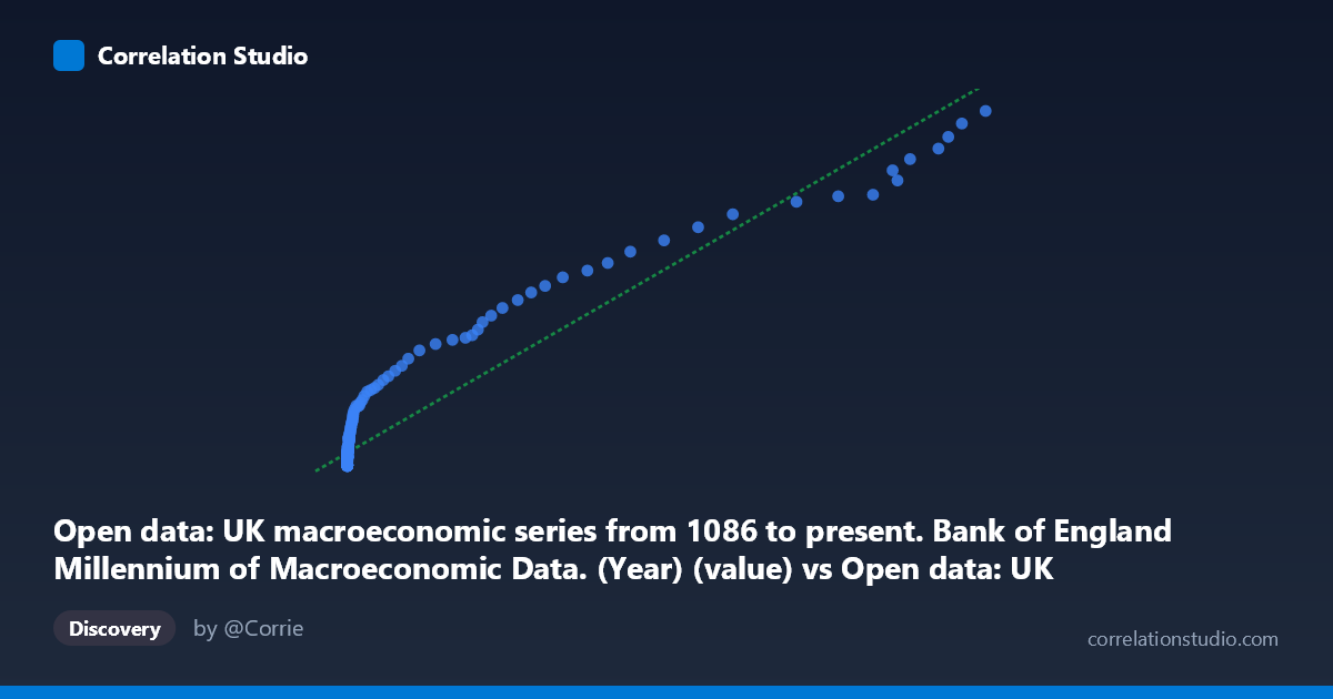
Open data: UK macroeconomic series from 1086 to present. Bank of England Millennium of Macroeconomic Data. (Year) (value) vs Open data: UK macroeconomic series from 1086 to present. Bank of England Millennium of Macroeconomic Data. (Month) (value)
- Pearson correlation (r)
- 0.9515
- Spearman correlation
- 0.9074
- p-value
- 0
- Sample size (n)
- 322
- 95% confidence interval
- 0.9399 to 0.9609
- Granger causality
- Bidirectional
- Granger optimal lag
- 10
AI analysis
Analysis of UK Macroeconomic Series: Annual vs. Monthly Value Correlation
Relationship Overview The scatterplot reveals a strong positive relationship between annual and monthly values drawn from the Bank of England's Millennium of Macroeconomic Data — a dataset spanning nearly a millennium of UK economic history. The linear regression equation (y = 5.1177x + 18,526) captures the broad trend, but the visualization makes clear that the relationship is not uniformly linear across the full range. At low X values (roughly below 500), there is a dense cluster of points near the origin with relatively modest Y values, while at higher X values the data fans outward into a more dispersed, elongated pattern characteristic of heteroscedasticity. This structural feature suggests the two measurement frequencies (annual vs. monthly) behave quite differently at different scales or time periods.
Correlation Strength and Statistical Significance The Pearson correlation of r = 0.9515 is exceptionally strong, and the R² of 0.9053 means that approximately 90.5% of the variance in monthly values is statistically explained by annual values across this sample. The 95% confidence interval [0.9399, 0.9609] is narrow, reflecting high precision in the estimate given the large population (N = 22,487) and paired sample (n = 322). The p-value of effectively zero confirms this is not a chance finding. The Granger causality results add meaningful nuance: bidirectional causality is detected at an optimal lag of 10 periods, meaning annual values help predict future monthly values (F = 3.008, p = 0.0012) and monthly values help predict future annual values (F = 2.714, p = 0.0034). While statistically significant, the F-statistics are modest, suggesting the predictive power in each direction — while real — is not overwhelming. This bidirectionality is consistent with both series being driven by underlying economic dynamics rather than one cleanly causing the other.
Notable Patterns, Clusters, and Outliers The sample points reveal at least two distinct behavioral regimes. The overwhelming majority of observations cluster tightly in the lower-left corner of the chart, with X values below ~200 and Y values below ~40,000 — likely corresponding to pre-industrial or early modern periods when macroeconomic magnitudes were small. A smaller but visually dominant group of points (e.g., X ≈ 91,374, Y ≈ 452,251; X ≈ 83,669, Y ≈ 405,374; X ≈ 72,987, Y ≈ 356,380) occupies the extreme upper-right and appears to represent modern-era high-value series such as nominal GDP, money supply, or equity indices measured in contemporary pound values. These high-leverage points likely drive much of the reported R², meaning the correlation is partly an artifact of scale differences across centuries rather than a tight functional relationship throughout the series.
Confounding Factors and Caveats Several important caveats apply. First, both axes draw from the same underlying dataset — the Bank of England Millennium database — meaning the correlation may partially reflect shared definitional or methodological conventions rather than an independent empirical finding. Second, the dataset aggregates hundreds of heterogeneous series (GDP, CPI, wages, interest rates, debt, equities), so the paired observations may be mixing economically unrelated quantities. Third, the extreme range in both X (3 to ~94,899) and Y (1,103 to ~468,775) spanning over 300 years introduces severe non-stationarity; correlations computed across such structurally different economic regimes can be misleading. The heteroscedasticity visible in the scatterplot — variance in Y clearly increasing with X — also violates a key assumption of ordinary linear regression, meaning the R² and regression coefficients should be interpreted cautiously.
Actionable Insights and Further Investigation To extract more meaningful insights, the analysis should be stratified by series type (e.g., price indices, output measures, financial variables) and by era (pre-industrial, industrial, post-WWII) to test whether the strong correlation holds within homogeneous subgroups or is driven purely by scale effects. A log-log transformation of both variables would likely linearize the relationship and stabilize variance, producing more interpretable regression parameters. Given the bidirectional Granger causality, investigating whether specific series (e.g., money supply leading prices) exhibit stronger directional predictability at varying lags would be economically informative. Finally, cointegration testing would be more appropriate than simple correlation for assessing long-run relationships between non-stationary macroeconomic time series of this kind.
X dataset: Open data: UK macroeconomic series from 1086 to present. Bank of England Millennium of Macroeconomic Data. (Month)
Y dataset: Open data: UK macroeconomic series from 1086 to present. Bank of England Millennium of Macroeconomic Data. (Year)
Part of experiment: Yearly - Open data: UK macroeconomic series from 1086 to present. Bank of England Millennium of Macroeconomic Data. (Month) vs Open data: UK macroeconomic series from 1086 to present. Bank of England Millennium of Macroeconomic Data. (Year)