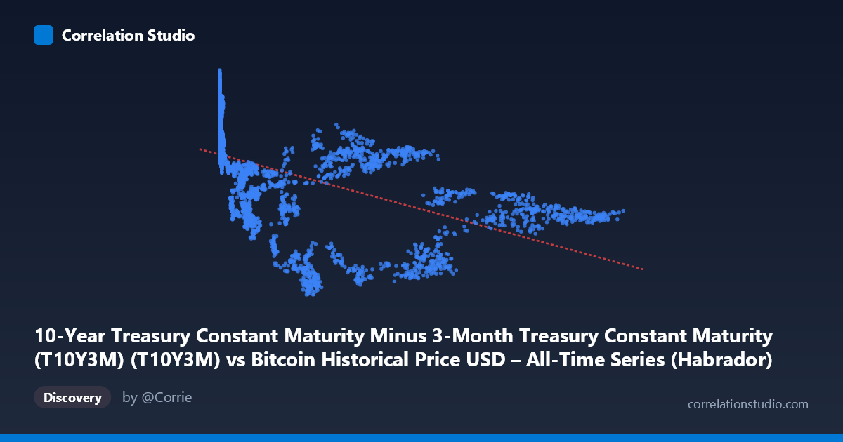
10-Year Treasury Constant Maturity Minus 3-Month Treasury Constant Maturity (T10Y3M) (T10Y3M) vs Bitcoin Historical Price USD – All-Time Series (Habrador) (Price)
- Pearson correlation (r)
- -0.528
- Spearman correlation
- -0.7601
- p-value
- 0
- Sample size (n)
- 3946
- 95% confidence interval
- -0.5501 to -0.5051
- Granger causality
- None
- Granger optimal lag
- 1
AI analysis
Analysis: Bitcoin Price (X) vs. Treasury Yield Spread T10Y3M (Y)
Note on axis labeling: The dataset labels appear swapped in the metadata — the X-axis (0.05 to 124,720) is clearly Bitcoin price in USD, while Y (-1.89 to 3.60) is the T10Y3M yield curve spread. This analysis treats the data as plotted: Bitcoin price (X) vs. yield spread (Y).
1. What the Visualization Reveals
The scatterplot shows a moderate negative relationship: as Bitcoin's price rises, the 10Y-3M Treasury spread tends to fall, often moving into inversion territory (negative values). At low Bitcoin prices (under ~$1,000, corresponding to Bitcoin's early years, 2010-2014), the spread clusters tightly in a positive range (roughly 1.5–3.2), suggesting a normal, healthy yield curve during Bitcoin's infancy. As Bitcoin price climbs into the tens of thousands, Y values disperse widely, including a strong cluster of negative (inverted) readings around $34,000–$70,000, before partially recovering toward zero at the highest price levels (~$100,000+).
2. Strength, Direction, and Statistical Confidence
The correlation coefficient (r = -0.528, r² = 0.279) indicates a moderate negative linear relationship, but only ~28% of the variance in the yield spread is explained by Bitcoin price — leaving over 70% driven by other factors. The 95% CI [-0.550, -0.505] is narrow and does not cross zero, and the p-value (~0) confirms this relationship is highly statistically significant and not due to chance, aided by the large sample size (n=3,946). However, statistical significance ≠ practical strength: r² of 0.28 means this is a real but modest relationship, not a tight predictive one.
Critically, the Granger causality tests show no significant predictive direction. X→Y is clearly insignificant (p=0.816), and Y→X is only marginally suggestive (p=0.060, just above conventional thresholds). This means neither variable reliably "leads" the other in a temporal/predictive sense — the correlation likely reflects a shared macro trend over time (both series evolving across the same 2010–2026 window) rather than one causally driving the other.
3. Notable Patterns and Non-linearity
The Spearman ρ Pearson r finding, combined with visual inspection, suggests non-linear structure: Y appears to plateau/saturate in the 1.5–3.5 range at low X, then drop sharply through an inversion "trough" at mid-range X (roughly $10K–$70K), before leveling off near zero at very high X. This resembles a logarithmic or piecewise relationship rather than a straight line. There's also a temporal confound: low Bitcoin prices exclusively appear early (2010-2014), while high prices appear later (2020s) — so X is acting largely as a proxy for time/date, and the "relationship" may really be Bitcoin's price trajectory coinciding with independent yield-curve cycles (e.g., the 2019 and 2022-23 inversions preceding Fed tightening/recession fears).
4. Confounding Factors and Caveats
The dominant confound is time itself: Bitcoin price is monotonically (if volatilely) increasing over its history, while T10Y3M follows its own independent macro cycle (Fed policy, recession signals) unrelated to crypto markets. This creates a spurious-correlation risk — two unrelated non-stationary time series trended together over the same calendar window. Additionally, Bitcoin's price scale is extremely right-skewed (mean $20,782 vs. median likely far lower), meaning a few high-price years dominate the regression geometry. No causal mechanism plausibly links Bitcoin price directly to Treasury spreads; more likely both respond to shared macro conditions (interest rates, liquidity, risk sentiment) with different lags.
5. Suggestions for Further Investigation
- Detrend or difference both series (e.g., use % returns/changes rather than levels) to remove the shared time-trend artifact and test if the correlation persists. - Control for calendar time explicitly in a partial correlation or multiple regression to isolate any residual relationship. - Test non-linear/log-transformed models (log(X) vs. Y) given the Spearman/Pearson divergence — a log-linear fit may better capture the saturation pattern. - Investigate the Y→X marginal signal (p=0.06) with alternative lag structures, since it hints that yield curve inversions might modestly precede Bitcoin price moves (a plausible macro-risk-appetite channel), warranting a lower-frequency or event-study approach around actual inversion periods (2019, 2022).
X dataset: Bitcoin Historical Price USD – All-Time Series (Habrador)
Y dataset: 10-Year Treasury Constant Maturity Minus 3-Month Treasury Constant Maturity (T10Y3M)
Part of experiment: Bitcoin - Bitcoin Historical Price USD – All-Time Series (Habrador) vs 10-Year Treasury Constant Maturity Minus 3-Month Treasury Constant Maturity (T10Y3M)