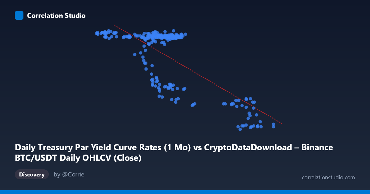
Daily Treasury Par Yield Curve Rates (1 Mo) vs CryptoDataDownload – Binance BTC/USDT Daily OHLCV (Close)

Pearson correlation (r): -0.749
Spearman correlation: -0.5349
p-value: 0
Sample size (n): 250
95% confidence interval: -0.7989 to -0.689
Granger causality: None
Granger optimal lag: 1

AI analysis

Analysis: Treasury Yield vs. BTC/USDT Close Price Relationship

1. What the Visualization Reveals

The scatterplot displays a clear negative, non-linear relationship between the two variables. As the "X" values (labeled Treasury 1-Month Par Yield but numerically ranging 39,568–106,133, which suggests a mislabeling — these values behave like price data) increase, the "Y" values (ranging 4.40–5.56) decline. The data appears to cluster into distinct regimes rather than following a smooth continuous trend: a dense cluster where X is between ~57,000–70,000 and Y sits high (5.4–5.55), and a second cluster where X exceeds ~85,000–100,000 with Y dropping sharply to 4.4–4.7. This bimodal clustering suggests two separate market regimes or time periods rather than one continuous linear process.

2. Strength, Direction, and Uncertainty

The correlation coefficient (r = -0.749) indicates a strong negative linear relationship, with r² = 0.561 meaning roughly 56% of the variance in Y is statistically explained by X — a substantial but incomplete relationship, leaving ~44% of variance driven by other factors. The 95% confidence interval [-0.799, -0.689] is tight and does not cross zero, and the p-value of ~0 confirms this correlation is highly statistically significant and not due to chance, given n=250. However, statistical significance and strength of correlation do not imply causation. The Granger causality tests reinforce this: neither direction (X→Y: F=0.605, p=0.437; Y→X: F=0.085, p=0.771) shows significant predictive power. This means that in a time-series sense, past values of one variable do not help forecast future values of the other — the relationship is contemporaneous/structural, not a lead-lag causal one.

3. Notable Patterns and Outliers

The data show a distinctly non-linear, almost step-like or threshold pattern rather than a smooth linear decay. The bulk of points cluster tightly at high Y (5.4–5.55) across a moderate X range, then a second cluster appears at much higher X values with sharply lower Y (~4.4–4.7). Intermediate points (e.g., X≈63,000–70,000, Y≈4.7–4.95) appear to bridge these clusters, suggesting a transition period. This pattern is more consistent with two regime states connected by a transitional period than a continuous linear relationship — the linear r² of 0.561 likely understates the strength of association within each regime and overstates it across the transition.

4. Confounders and Caveats

The variable labeling is inconsistent (X labeled as Treasury yield data, but described as BTC/USDT OHLCV; Y labeled as BTC close price, but range and dataset description point to Treasury yields) — this metadata mismatch should be resolved before drawing substantive economic conclusions. Additionally, both series are time-ordered financial/macro variables likely non-stationary (trending over the year), which can produce spurious correlation independent of any real relationship — this is a classic caveat for regressing two trending time series. The clustering pattern also suggests a hidden third variable (e.g., time regime, monetary policy shift, or market cycle phase) driving both series' comovement rather than one directly influencing the other.

5. Recommendations for Further Investigation

First, verify and correct the axis/column labeling to ensure the analysis reflects the intended variables. Second, given the non-stationarity typical of financial and rate data, run the correlation on differenced or returns-based series (ΔX, ΔY) rather than levels to check if the relationship holds or is spurious. Third, investigate the apparent regime clustering with a structural break test or by segmenting the year into sub-periods (e.g., by quarter) to see if the relationship is stable or driven by one specific period (e.g., a Fed rate-cut cycle coinciding with a BTC rally). Finally, since Granger causality found no predictive direction, consider testing for a contemporaneous common-driver model (e.g., macro liquidity conditions or risk sentiment) rather than treating this as a forecasting relationship.

X dataset: CryptoDataDownload – Binance BTC/USDT Daily OHLCV

Y dataset: Daily Treasury Par Yield Curve Rates

Part of experiment: Bitcoin - CryptoDataDownload – Binance BTC/USDT Daily OHLCV vs Daily Treasury Par Yield Curve Rates