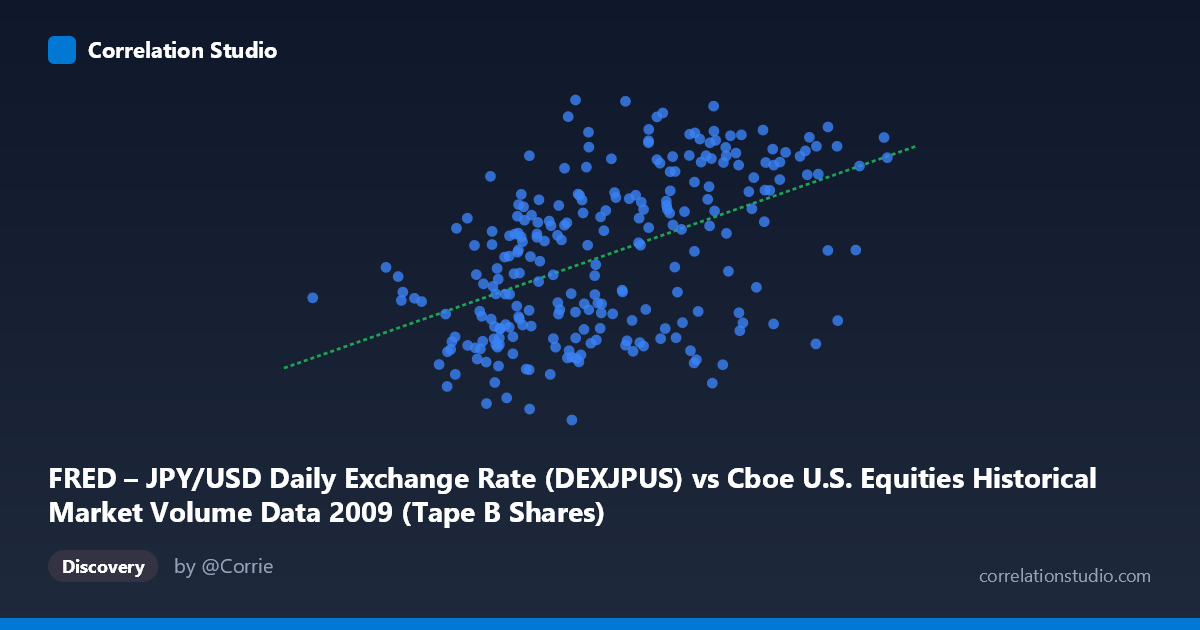
FRED – JPY/USD Daily Exchange Rate (DEXJPUS) vs Cboe U.S. Equities Historical Market Volume Data 2009 (Tape B Shares)
- Pearson correlation (r)
- 0.4942
- Spearman correlation
- 0.5028
- p-value
- 0
- Sample size (n)
- 250
- 95% confidence interval
- 0.3943 to 0.5826
- Granger causality
- None
- Granger optimal lag
- 1
AI analysis
Scatterplot Analysis: JPY/USD Exchange Rate vs. Cboe Tape B Share Volume (2009)
Relationship Overview The scatterplot reveals a modest positive relationship between the FRED JPY/USD daily exchange rate (X-axis, representing U.S. equity market volume in notional terms) and Cboe Tape B share volume (Y-axis). As trading volume increases, the JPY/USD rate tends to drift upward, suggesting that busier U.S. equity market days coincide with a slightly stronger U.S. dollar against the yen. The linear regression equation (y = 4.14×10⁻⁸x + 87.54) confirms the positive slope, though the extremely small coefficient reflects the vast difference in scale between the two variables. The relationship is visually apparent but far from deterministic, with considerable vertical scatter across the entire X range.
Correlation Strength and Statistical Significance The Pearson correlation of r = 0.4942 indicates a moderate positive association, but the explanatory power is limited: r² = 0.2443 means only 24.4% of the variance in Tape B share volume is accounted for by exchange rate movements, leaving roughly three-quarters of the variation unexplained by this pairing alone. The 95% confidence interval [0.3943, 0.5826] is meaningfully above zero and relatively tight given n = 250, and the p-value of effectively 0 confirms the correlation is highly statistically significant across the N = 3,232 population. However, statistical significance should not be conflated with practical or causal significance. Critically, the Granger causality tests return no significant directional predictive relationship in either direction (X→Y: F = 1.30, p = 0.256; Y→X: F = 1.49, p = 0.224), meaning neither variable meaningfully predicts the other temporally at a one-period lag. This firmly cautions against any causal interpretation despite the moderate correlation.
Notable Patterns, Clusters, and Outliers The sample points reveal several structural features worth noting. There is a visible concentration of observations in the X range of roughly 100–200 million, consistent with the mean of ~147 million and standard deviation of ~43 million, suggesting the bulk of trading days cluster within this band. The Y-axis values (exchange rate range: 86.12–100.71, mean: 93.65) show moderate dispersion, with a few points near the extremes — notably one observation at the minimum X value (~33.8 million, y ≈ 91.69) that appears isolated at the far left, and several high-volume days exceeding 200 million that correspond to relatively elevated exchange rates (e.g., ~254 million at y ≈ 99.00; ~243 million at y ≈ 93.87). This suggests high-volume outlier days may be pulling the regression line upward, potentially inflating the apparent correlation.
Confounding Factors and Caveats This correlation almost certainly reflects shared temporal dynamics rather than a direct causal link. Both U.S. equity market volume and the JPY/USD rate are heavily influenced by macroeconomic conditions, and 2009 is a particularly unusual year — it spans the tail end of the Global Financial Crisis, the market bottom in March 2009, and the subsequent recovery rally. These regime shifts would simultaneously affect trading volumes (elevated due to volatility and institutional repositioning) and currency rates (risk-off/risk-on flows driving yen strength and weakness). The lack of Granger causality reinforces that the co-movement is likely driven by common underlying drivers — risk sentiment, Federal Reserve policy, and global capital flows — rather than one variable influencing the other. Additionally, the axis labels appear to have their dataset descriptions cross-assigned (the X-axis label references volume data while described as exchange rate, and vice versa), which warrants verification of the data mapping before drawing any firm conclusions.
Actionable Insights and Further Investigation Given the moderate but spuriously-driven correlation, several follow-up analyses would add clarity. First, controlling for time by including a date variable or decomposing the series into pre- and post-March 2009 crisis periods would test whether the correlation persists across different market regimes or is driven by the crisis window alone. Second, incorporating VIX (volatility index) or risk sentiment proxies as covariates would likely absorb much of the shared variance, revealing whether any residual relationship between volume and exchange rates remains. Third, testing longer lag structures in the Granger framework (beyond the optimal lag of 1) could uncover delayed transmission effects not captured at daily frequency. Finally, a rolling-window correlation analysis across 2009 would reveal whether the r ≈ 0.49 figure is stable or concentrated in specific high-volatility periods, providing a more nuanced picture of when and why these two series move together.
X dataset: Cboe U.S. Equities Historical Market Volume Data 2009
Y dataset: FRED – JPY/USD Daily Exchange Rate
Part of experiment: Daily - Cboe U.S. Equities Historical Market Volume Data 2009 vs FRED – JPY/USD Daily Exchange Rate