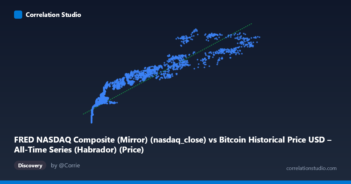
FRED NASDAQ Composite (Mirror) (nasdaq_close) vs Bitcoin Historical Price USD – All-Time Series (Habrador) (Price)
- Pearson correlation (r)
- 0.9293
- Spearman correlation
- 0.9815
- p-value
- 0
- Sample size (n)
- 3970
- 95% confidence interval
- 0.925 to 0.9335
- Granger causality
- None
- Granger optimal lag
- 10
- Time coverage
- 2010-07-19 to 2026-04-28
AI analysis
Analysis: Bitcoin Price vs. NASDAQ Composite
1. Relationship Overview
The scatterplot depicts a strong, positive, non-linear relationship between NASDAQ Composite levels (X) and Bitcoin's USD price (Y). Rather than a clean straight-line pattern, the data show a curved, compressed relationship at low X-values that flattens and stretches at higher X-values — consistent with the underlying data-generating process: Bitcoin's early history (near-zero prices, $0.05–$100 range) coincided with a NASDAQ that was already trading in the thousands, so the low end of the X range maps to a tight vertical cluster in Y (~$2,100–$4,000). As X increases into the tens of thousands, Y spreads out dramatically, ranging from roughly $6,000 to nearly $25,000. This produces a logarithmic-looking curve rather than a linear one.
2. Strength, Direction, and Statistical Meaning
The Pearson correlation (r = 0.929) is very strong and positive, and r² = 0.864 indicates that roughly 86% of the variance in Y is statistically associated with X in a linear framework. The 95% CI [0.925, 0.933] is tight given the large sample (n=3,970), and the p-value of ~0 confirms this correlation is not due to random chance. However, correlation strength should not be mistaken for causal or predictive power: the Granger causality tests show no significant predictive direction in either direction (X→Y: p=0.89; Y→X: p=0.80) even at an optimal lag of 10 periods. This is a critical caveat — the strong contemporaneous correlation is likely driven by a shared underlying trend (both assets generally appreciated over the 2010–2026 window) rather than one variable mechanically forecasting the other. In practice, this means the relationship is descriptive/co-trending, not a reliable trading or forecasting signal.
3. Notable Patterns and Outliers
Several features stand out: - Compressed low-X cluster: A large mass of points sits at X < 1,000 with Y values in the $2,500–$6,000 band — this reflects Bitcoin's multi-year "flat" era relative to NASDAQ's already-elevated baseline. - Curvature/heteroscedasticity: Variance in Y increases substantially as X grows (e.g., at X≈86,000–98,000, Y ranges from ~$18,300 to ~$23,500), suggesting the true relationship is closer to log-linear or power-law than the fitted linear model (y = 0.177x + 5,269) captures well at the extremes. - Divergence at high X: Points like (86,475, 18,350) vs. (86,473, 23,276) show two very different Y values for nearly identical X — a sign that time-lag effects, volatility clustering, or regime shifts (bull/bear cycles) are driving Y independently of X at times. - No extreme leverage outliers, but the tails (very low and very high X) exert disproportionate influence on the linear fit.
4. Confounding Factors and Caveats
The most important caveat: both series exhibit strong secular time trends (both broadly rose 2010–2026), which can inflate correlation without implying any direct economic link — a classic case of "spurious correlation via co-trending non-stationary time series." Neither series is likely stationary, and standard Pearson correlation on trending data can overstate the relationship's meaningfulness. Additionally, macro factors (global liquidity/interest rates, risk-on/risk-off sentiment, USD strength) plausibly drive both tech equities and Bitcoin simultaneously, acting as a lurking confounder rather than one asset causing the other. Data granularity/misalignment (daily NASDAQ vs. Bitcoin's 24/7 trading) and the linear model's poor fit at scale extremes further limit interpretability.
5. Suggestions for Further Investigation
- De-trend or difference both series (e.g., use log returns instead of levels) and recompute correlation/Granger tests — this is essential to rule out spurious correlation from shared trends. - Test for cointegration (e.g., Engle-Granger or Johansen test) given both series are likely non-stationary; this would clarify whether a genuine long-run equilibrium relationship exists. - Fit a log-log or power-law model instead of linear regression, given the visible curvature — likely to substantially improve fit and interpretability. - Segment by market regime (bull vs. bear cycles, pre/post major halving events) to see if the relationship strength or slope changes over time. - Treat the current r²/r results as descriptive of historical co-movement, not as a basis for predictive modeling, given the null Granger causality result.
X dataset: Bitcoin Historical Price USD – All-Time Series (Habrador)
Y dataset: FRED NASDAQ Composite (Mirror)
Part of experiment: Bitcoin - Bitcoin Historical Price USD – All-Time Series (Habrador) vs FRED NASDAQ Composite (Mirror)