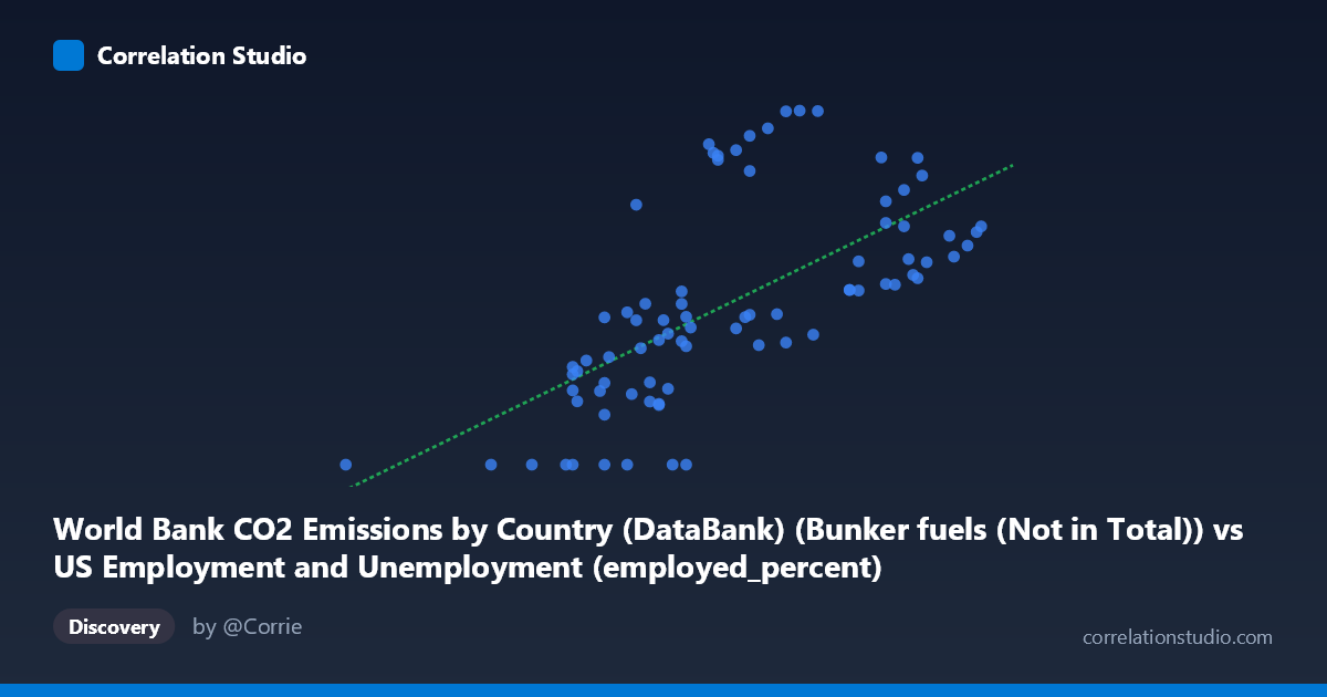
World Bank CO2 Emissions by Country (DataBank) (Bunker fuels (Not in Total)) vs US Employment and Unemployment (employed_percent)
- Pearson correlation (r)
- 0.6493
- Spearman correlation
- 0.7367
- p-value
- 0
- Sample size (n)
- 80
- 95% confidence interval
- 0.5011 to 0.7605
- Granger causality
- None
- Granger optimal lag
- 10
- Time coverage
- 1941-01-01 to 2020-01-01
AI analysis
Scatterplot Analysis: Bunker Fuel CO₂ Emissions vs. US Employment Percentage
1. Overall Relationship Revealed
The scatterplot reveals a moderate positive relationship between global bunker fuel CO₂ emissions (X-axis, measured in units spanning roughly 50–65) and US employment percentage (Y-axis, ranging from 0 to ~1,592). The linear regression equation y = 99.31x − 5,118.33 suggests that for each unit increase in bunker fuel emissions, the employed percentage rises by approximately 99 units. Visually, the data points show a general upward trend from lower-left to upper-right, but with considerable vertical scatter — particularly in the mid-range of X values (56–60), where Y values span nearly the full range from 0 to 1,500+. This wide dispersion signals that the relationship, while real, is far from deterministic.
2. Correlation Strength, Direction, and Causality
The Pearson correlation of r = 0.649 indicates a moderate positive association, and the R² of 0.422 means that bunker fuel emissions statistically explain roughly 42% of the variance in US employment percentage — a meaningful but decidedly incomplete picture, with 58% of variation attributable to other factors. The 95% confidence interval for r of [0.501, 0.761] is encouragingly narrow and sits entirely above zero, reinforcing genuine statistical confidence in the positive direction. The p-value of 7.27×10⁻¹¹ is extraordinarily small, making chance alone an implausible explanation across the N=80 paired observations spanning 1941–2020.
However, the Granger causality results critically undermine any causal narrative: neither direction (X→Y: F=1.03, p=0.431; Y→X: F=1.49, p=0.172) reaches statistical significance, even at an optimal lag of 10 periods. This means that past values of bunker fuel emissions do not improve prediction of future US employment levels, and vice versa. The correlation is real, but temporal predictive power is absent — a hallmark of spurious or confounded correlation driven by shared underlying trends rather than genuine causal linkage.
3. Notable Patterns, Clusters, and Outliers
Several notable features stand out in the data:
- Vertical striping and clustering is visible around X ≈ 56–58, where many data points pile up across the full Y range, suggesting these emission values occurred across many different years with vastly different employment contexts. - A cluster of zero-value Y observations (at least 8–9 points where Y = 0.00, e.g., at X = 57.9, 55.4, 57.6, 50.4, 53.6, 56.1, 54.5, 56.6) is particularly suspicious — these likely represent missing data coded as zero rather than genuine zero employment percentages, which would be economically impossible. - High-Y outliers around X = 59.3 (Y ≈ 1,478), X = 60.4 (Y ≈ 1,592), and X = 60.8 (Y ≈ 1,590) pull the regression line upward and may disproportionately inflate the correlation. - The upper range of X (62–64) shows a tighter, more consistent clustering of moderate-to-high Y values, suggesting the relationship may be stronger at higher emission levels. - There is a possible non-linear or threshold pattern, where the relationship appears weaker or more scattered at lower X values and somewhat more structured at higher X values.
4. Confounding Factors and Caveats
This correlation warrants serious interpretive caution for several reasons:
- Spurious long-run trends: Both bunker fuel emissions and US employment have generally increased over the 1941–2020 period due to global economic growth and post-WWII industrialization. Two variables sharing an upward secular trend will correlate even without any direct connection — this is the classic "third variable" or common-trend problem. - Zero-coded missing data: The multiple Y = 0.00 values almost certainly represent missing or unreported data rather than actual employment figures, artificially distorting both the regression and correlation estimates. - Dataset mismatch: The X variable comes from a "US Employment and Unemployment" dataset but represents global bunker fuel emissions, while the Y variable comes from a "World Bank CO₂ Emissions" dataset but represents US employment percentage — suggesting these columns may have been inadvertently swapped or cross-joined, raising serious data integrity concerns. - Aggregation level mismatch: Annual bunker fuel emissions (a global maritime/aviation metric) and national employment rates operate at fundamentally different scales and mechanisms, making direct mechanistic interpretation difficult. - The Granger null result at 10 lags further confirms no predictive temporal structure connects these series beyond their shared trend.
5. Actionable Insights and Further Investigation
Given the significant caveats, the following steps are recommended:
1. Audit the data pipeline: Verify that X and Y columns were correctly extracted from their respective datasets — the dataset/column label crossover is a red flag for a data join or labeling error that would invalidate the entire analysis. 2. Address zero-coded values: Remove or impute the Y = 0.00 observations after confirming they represent missing data; re-run the correlation and regression to assess how much the r value changes. 3. Detrend both series: Apply first-differencing or HP-filtering to remove shared long-run trends before re-examining correlation, which would test whether a cyclical relationship (beyond secular growth) exists. 4. Explore the high-X cluster: Investigate whether the stronger apparent relationship at X 62 corresponds to specific decades (likely post-2000) and whether other global economic variables (GDP, trade volume) better explain the clustering. 5. Consider multivariate modeling: If a genuine research question exists linking maritime emissions to labor markets, introduce control variables such as global GDP, oil prices, and trade volumes to isolate any conditional relationship between these two metrics.
X dataset: US Employment and Unemployment
Y dataset: World Bank CO2 Emissions by Country (DataBank)
Part of experiment: Yearly - US Employment and Unemployment vs World Bank CO2 Emissions by Country (DataBank)