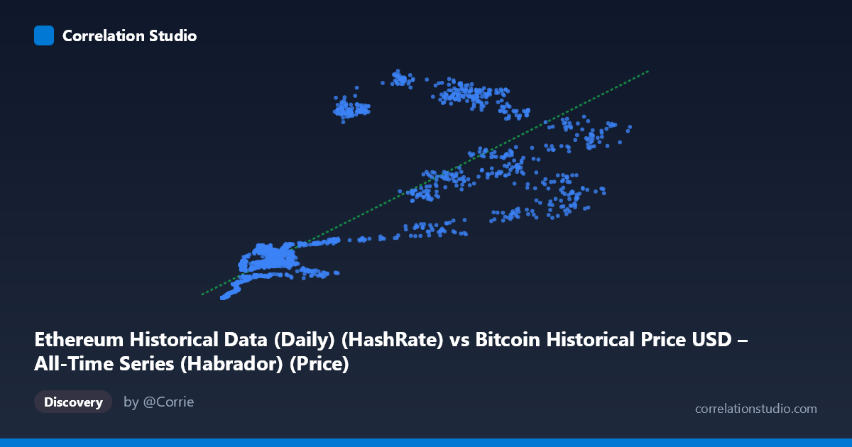
Ethereum Historical Data (Daily) (HashRate) vs Bitcoin Historical Price USD – All-Time Series (Habrador) (Price)
- Pearson correlation (r)
- 0.8175
- Spearman correlation
- 0.91
- p-value
- 0
- Sample size (n)
- 2604
- 95% confidence interval
- 0.8044 to 0.8299
- Granger causality
- None
- Granger optimal lag
- 1
- Time coverage
- 2015-07-30 to 2022-09-14
- Recomputed on refreshed data
- 2026-10-24 (r was 0.8175)
AI analysis
Analysis: Ethereum Hash Rate vs. Bitcoin Price Relationship
1. What the Visualization Reveals
The scatterplot depicts a strong positive relationship between the labeled "hash rate" variable (X) and price variable (Y), with values climbing together across the full range. At low X values (roughly 200–3,000), Y clusters tightly near zero (0.08–20), while at high X values (40,000–65,000+), Y climbs into the 500–1,065 range. The pattern is not perfectly linear — it shows an accelerating, convex shape typical of two variables that both trend upward over time (e.g., both driven by market growth/adoption cycles) rather than a mechanistic linear coupling. Note the column labels appear swapped/mismatched in the metadata (X is described as Ethereum HashRate but titled "Bitcoin Price," and Y vice versa) — this should be verified before drawing domain-specific conclusions.
2. Strength, Direction, and Uncertainty
The correlation coefficient (r = 0.8175) indicates a strong positive linear association, with r² = 0.6683 meaning roughly 67% of the variance in Y is statistically explained by X — a substantial but incomplete fit, leaving about a third of Y's variance driven by other factors. The 95% CI [0.8044, 0.8299] is tight, and p ≈ 0 confirms this correlation is highly unlikely to be due to chance given the large sample (n=2,604). However, correlation strength should not be conflated with causation: the Granger causality tests show no significant predictive direction in either direction (X→Y: p=0.40; Y→X: p=0.31). This is a critical finding — despite the strong contemporaneous correlation, neither variable helps forecast the other's future values based on past values. This pattern is classic for two series that are both driven by a common underlying trend (e.g., overall crypto market growth, adoption, or time itself) rather than one causally driving the other.
3. Notable Patterns and Outliers
Several features stand out: - Heteroscedasticity: Variance in Y increases sharply as X increases — low-X points are tightly clustered near zero, while high-X points spread widely (e.g., at X≈20,000, Y ranges from 845 to 927; at X≈48,000–56,000, Y ranges from 456 to 1,017). This fanning pattern suggests the linear model underperforms at higher values. - Possible regime clusters: Points like (20,381, 927.30), (20,212, 845.85), (29,047, 1,017.23), and (48,610, 874.30) sit well above the regression line's prediction, suggesting a secondary regime or period (possibly a specific bull market phase) where Y was elevated relative to X. - Compression at low end: Below X=1,000, Y is compressed near zero, indicating a possible floor/threshold effect or measurement granularity issue at small values. - A negative-residual outlier: (56,234, 456.86) sits notably below where the trend would predict, given nearby points like (48,610, 874.30) and (65,199, 812.84).
4. Confounding Factors and Caveats
Both variables span 2015–2022, a period encompassing multiple crypto bull/bear cycles — time itself is a likely confounder, as both hash rate/network activity and price tend to trend upward over long horizons due to broader adoption, independent of any direct causal link. Autocorrelation within each time series (both are highly serially correlated, non-stationary trends) inflates the apparent correlation and violates independence assumptions underlying standard significance tests — the p-value near zero should be interpreted cautiously for this reason. Additionally, macro factors (regulatory news, exchange listings, broader market sentiment, mining difficulty adjustments) likely affect both series simultaneously, and the labeling ambiguity between Bitcoin/Ethereum price/hashrate columns needs resolution to ensure the causal narrative fits the actual variables being compared.
5. Actionable Insights
- Verify column labeling before publishing conclusions, given the apparent mismatch between axis titles and dataset descriptions. - Detrend or difference both series (e.g., use returns/percentage changes rather than levels) and re-run correlation and Granger tests — this often reveals whether the relationship holds beyond shared trend, or whether it's an artifact of both series moving together over time. - Test a log-log or power-law model given the convex, heteroscedastic pattern — this may substantially improve fit over the current linear model (R²=0.668). - Segment by time period (e.g., by bull/bear cycle) to check whether the strong high-Y outliers (2020–2021 bull run) are driving the overall correlation, and whether the relationship is weaker/absent in other periods. - Given the lack of Granger causality, avoid using one series to forecast the other in trading or predictive models; instead, investigate shared external drivers (e.g., overall market cap, trading volume, or investor sentiment indices) as the true causal mechanism linking both variables.
X dataset: Bitcoin Historical Price USD – All-Time Series (Habrador)
Y dataset: Ethereum Historical Data (Daily)
Part of experiment: Bitcoin - Bitcoin Historical Price USD – All-Time Series (Habrador) vs Ethereum Historical Data (Daily)