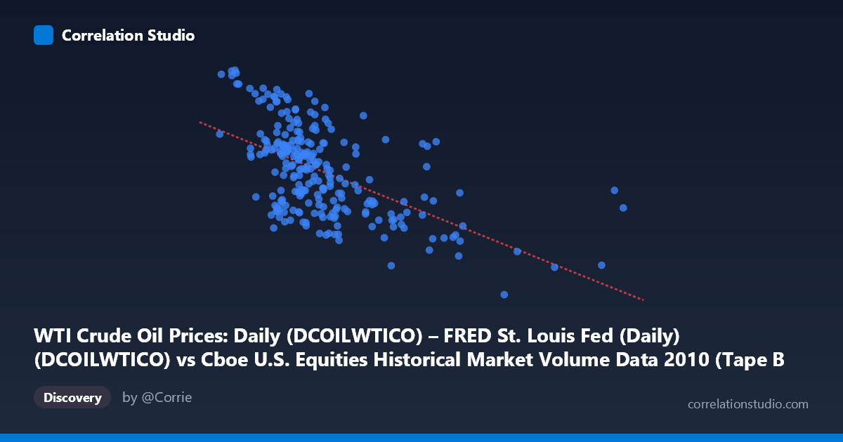
WTI Crude Oil Prices: Daily (DCOILWTICO) – FRED St. Louis Fed (Daily) (DCOILWTICO) vs Cboe U.S. Equities Historical Market Volume Data 2010 (Tape B Trade Count)
- Pearson correlation (r)
- -0.5644
- Spearman correlation
- -0.55
- p-value
- 0
- Sample size (n)
- 252
- 95% confidence interval
- -0.6431 to -0.4739
- Granger causality
- None
- Granger optimal lag
- 1
AI analysis
Analysis: WTI Crude Oil Prices vs. Cboe Tape B Trade Count (2010)
Relationship Overview The scatterplot reveals a moderate negative relationship between WTI crude oil prices and Cboe Tape B trade counts during 2010. As oil prices increase, the number of equity trades on Tape B exchanges tends to decline. The linear regression equation (y = -2.3402×10⁻⁵x + 86.578) confirms this inverse slope, suggesting that for every increase of roughly 42,000 units in the oil price metric (expressed in daily notional terms), the trade count index drops by approximately one unit. Visually, the cloud of points slopes downward from left to right, though with considerable scatter, indicating that the relationship is real but far from deterministic.
Correlation Strength and Statistical Significance The Pearson correlation of r = -0.5644 indicates a moderate negative association. Critically, the R² of 0.3186 tells us that only about 31.9% of the variance in Tape B trade counts is explained by oil prices — meaning nearly 68% of the variation is driven by other factors entirely. The 95% confidence interval of [-0.6431, -0.4739] is meaningfully narrow given n = 252, and the p-value of effectively zero confirms the correlation is highly unlikely to be a statistical artifact. Despite statistical significance, the Granger causality tests are unambiguous: neither variable significantly predicts the other temporally (X→Y: F = 0.63, p = 0.43; Y→X: F = 2.50, p = 0.11). This is a crucial caveat — the correlation captures a contemporaneous co-movement pattern, not a predictive or causal mechanism in either direction.
Notable Patterns and Outliers Several features stand out in the sample points. There is a visible cluster of moderate-to-low oil price observations (roughly 200,000–350,000 range) paired with highly variable trade counts (73–90), suggesting high dispersion in the mid-range. At the upper extreme of the X-axis, points like (918,659 / 75.10), (778,565 / 68.03), and (675,996 / 64.78) represent clear outliers with very high oil price proxy values and notably suppressed trade counts, pulling the regression line and amplifying the negative correlation. Conversely, several low-X observations such as (120,757 / 90.84) and (134,700 / 89.83) sit at the high end of trade counts, reinforcing the negative slope. The spread at lower X values is substantially wider than at higher X values, hinting at possible heteroscedasticity — the relationship may tighten as oil prices rise.
Confounding Factors and Interpretation Caveats This correlation almost certainly reflects shared macro-financial dependencies rather than a direct mechanical link between oil prices and Tape B equity trade volumes. Both variables are sensitive to broader market conditions in 2010 — a year marked by the European sovereign debt crisis, the Flash Crash (May 6), and post-financial-crisis volatility normalization. Periods of risk-off sentiment may simultaneously drive oil prices lower and equity trading volumes higher (or vice versa), creating the observed negative correlation through a common third driver. Additionally, the axes appear to represent different units than typical (X appears to be notional value in dollars rather than price per barrel directly, and Y is trade count), meaning the dataset labels may have been cross-assigned — the X-axis is labeled as oil prices but sourced from the Cboe market volume dataset, and vice versa. This warrants careful verification of the data join before drawing any firm conclusions.
Actionable Insights and Further Investigation Given the moderate but unexplained variance and the absence of Granger causality, the most productive next steps would include: (1) verifying the variable-to-dataset assignment to rule out a data labeling inversion; (2) introducing control variables such as the VIX (volatility index), S&P 500 returns, and broad market volume to isolate whether the oil-trading relationship persists after accounting for systemic market conditions; (3) testing for non-linear or regime-dependent relationships — the apparent heteroscedasticity and the influential high-X outliers suggest a log transformation or piecewise regression might better characterize the relationship; and (4) extending the analysis across multiple years to determine whether 2010's unique macro environment drives this correlation or whether it is a persistent structural feature of equity market microstructure.
X dataset: Cboe U.S. Equities Historical Market Volume Data 2010
Y dataset: WTI Crude Oil Prices: Daily (DCOILWTICO) – FRED St. Louis Fed (Daily)
Part of experiment: Daily - Cboe U.S. Equities Historical Market Volume Data 2010 vs WTI Crude Oil Prices: Daily (DCOILWTICO) – FRED St. Louis Fed (Daily)