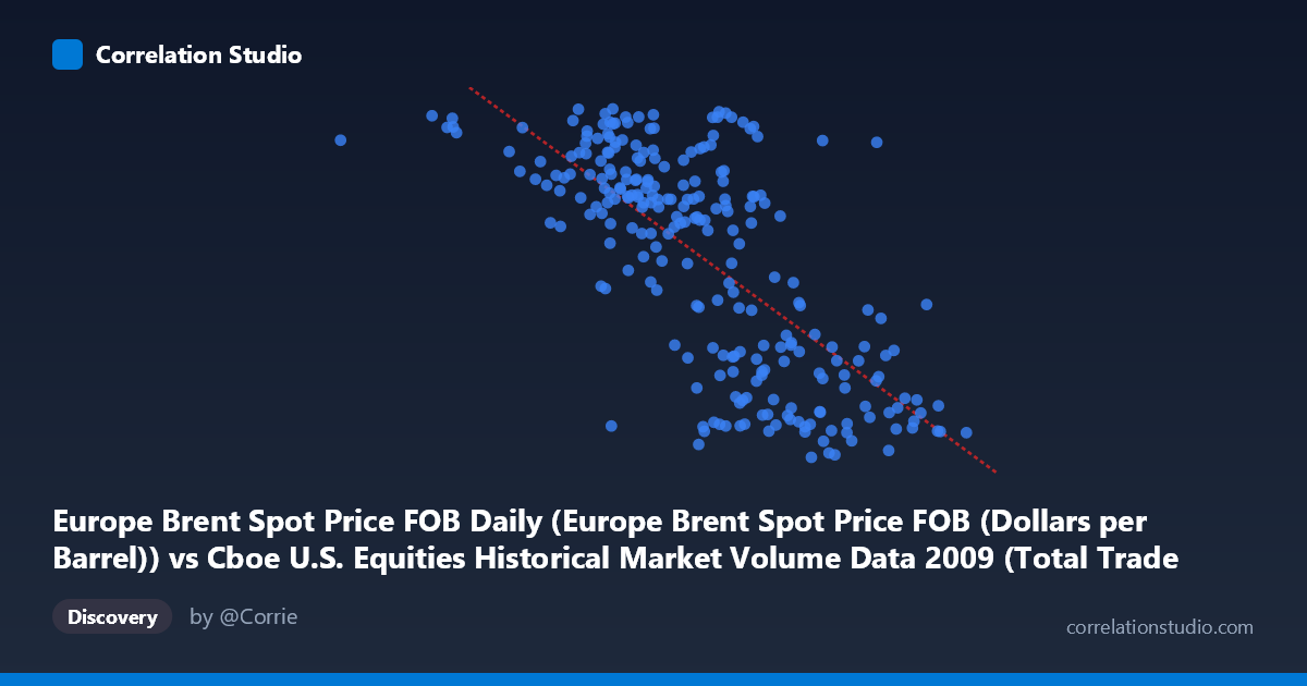
Europe Brent Spot Price FOB Daily (Europe Brent Spot Price FOB (Dollars per Barrel)) vs Cboe U.S. Equities Historical Market Volume Data 2009 (Total Trade Count)
- Pearson correlation (r)
- -0.7138
- Spearman correlation
- -0.6969
- p-value
- 0
- Sample size (n)
- 252
- 95% confidence interval
- -0.7695 to -0.6473
- Granger causality
- None
- Granger optimal lag
- 1
AI analysis
Analysis: Europe Brent Spot Price vs. U.S. Equities Total Trade Count (2009)
Relationship Overview The scatterplot reveals a negative relationship between Europe Brent Spot Price (X) and U.S. Equities Total Trade Count (Y) across 2009. As oil prices rise, equity trade counts tend to decline, and vice versa. The linear regression equation (y = −1.47×10⁻⁵x + 100.97) captures this downward slope across the data cloud. This pattern is visually coherent — lower oil price periods (roughly corresponding to early 2009 recovery phases) coincide with elevated trading activity, while higher oil price readings cluster toward lower trade counts. The relationship is consistent enough to be meaningful but with notable scatter, suggesting other forces are simultaneously at work.
Correlation Strength and Statistical Significance The Pearson correlation of r = −0.714 indicates a moderately strong negative association. More concretely, r² = 0.509 means that roughly 51% of the variance in trade count is statistically explained by variation in Brent oil prices — a substantial but far from complete explanation. The 95% confidence interval of [−0.770, −0.647] is notably narrow and lies entirely in negative territory, confirming that the direction of the relationship is robust and not a sampling artifact. The p-value of essentially zero, combined with a sample of n = 252 drawn from a population of N = 3,232, provides strong statistical confidence. However, the Granger causality tests tell a critical story: neither X→Y (F = 0.322, p = 0.571) nor Y→X (F = 1.222, p = 0.270) achieves significance at any conventional threshold. This means that despite the strong contemporaneous correlation, neither variable reliably predicts the other one period ahead — the relationship is associative, not temporally directional.
Notable Patterns, Clusters, and Outliers The data exhibits two visually distinct clusters. One cluster sits at higher trade counts (roughly Y = 65–78) paired with lower oil prices (X ≈ 629K–2.5M range), while a second denser cluster occupies lower trade counts (Y ≈ 40–55) at higher oil price levels (X ≈ 2.8M–4.1M). The point at approximately (629,671, 75.15) stands out as an extreme outlier on the low end of X, potentially representing a very low-volume trading day or a data anomaly. Several high-X points near (4,134,003, 42.19) and (3,911,469, 56.63) anchor the upper oil price boundary. The scatter is somewhat heteroscedastic — variance in Y appears larger at intermediate X values — and there may be a mild non-linear (concave) curvature, suggesting a linear model slightly oversimplifies the true functional form.
Confounding Factors and Caveats This correlation almost certainly reflects shared temporal dynamics rather than a direct causal mechanism. Both variables are time series from 2009 — a year dominated by the post-financial crisis recovery — and both were heavily influenced by the same macro forces: the March 2009 market bottom, the subsequent global equity rally, and the concurrent rebound in oil demand and prices. This creates a classic spurious correlation via common cause: improving economic conditions drove equity volumes down as panic selling abated while simultaneously driving oil prices up. Additionally, the axis labeling warrants scrutiny — the dataset descriptions appear to have the column assignments swapped (Brent price data is attributed to the Cboe volume dataset and vice versa), which could reflect a metadata issue requiring verification before formal reporting.
Actionable Insights and Further Investigation Given that Granger causality is absent, traders and analysts should not use Brent oil prices as a leading indicator for equity trade counts (or vice versa) in short-term tactical models at a one-day lag. Instead, both variables should be modeled as co-dependent responses to underlying macro conditions. Recommended next steps include: (1) introducing a macro control variable such as VIX or GDP growth rate to test whether the correlation weakens or disappears after conditioning; (2) testing non-linear models (e.g., polynomial or piecewise regression) given the visual suggestion of curvature; (3) verifying the dataset column assignments to ensure X and Y are correctly mapped; and (4) extending the Granger analysis to longer lags (2–5 periods) and to other years to determine whether the null result is specific to 2009's unusual market dynamics or a general property of this variable pair.
X dataset: Cboe U.S. Equities Historical Market Volume Data 2009
Y dataset: Europe Brent Spot Price FOB Daily
Part of experiment: Daily - Cboe U.S. Equities Historical Market Volume Data 2009 vs Europe Brent Spot Price FOB Daily