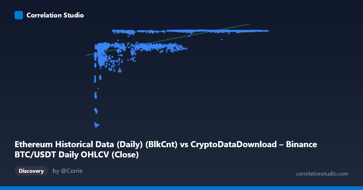
Ethereum Historical Data (Daily) (BlkCnt) vs CryptoDataDownload – Binance BTC/USDT Daily OHLCV (Close)

Pearson correlation (r): 0.5729
Spearman correlation: 0.7308
p-value: 0
Sample size (n): 3191
95% confidence interval: 0.5491 to 0.5957
Granger causality: None
Granger optimal lag: 1
Time coverage: 2017-08-17 to 2026-05-20

AI analysis

Analysis of Ethereum Block Count vs. BTC/USDT Close Price Relationship

1. What the visualization reveals

The scatterplot shows a moderate positive relationship between the X variable (labeled as Ethereum block count, though the value ranges — thousands to ~124,000 — and behavior suggest this may actually be a mislabeled volume or transaction-count metric) and the Y variable (BTC/USDT closing price). The data does not form a tight linear band; instead, it displays a curved, saturating pattern: Y rises steeply as X increases from its minimum (~3,000) up to roughly 20,000–30,000, then plateaus and flattens between 7,100–7,180 for the remainder of the X range (up to 124,000). This is characteristic of a logarithmic or square-root relationship rather than a straight line.

2. Strength, direction, and statistical confidence

The Pearson correlation (r = 0.573) indicates a moderate positive linear association, with r² = 0.328 meaning the linear model explains only about 33% of the variance in Y — leaving two-thirds unexplained by a straight-line fit. The 95% CI [0.549, 0.596] is narrow, and the p-value is effectively 0, so we can be highly confident a real, non-zero linear relationship exists in this sample; the uncertainty here concerns effect size interpretation, not statistical significance. Critically, the note that Spearman's ρ exceeds Pearson's r confirms what the scatterplot shows visually: the true relationship is monotonic but non-linear, so a log or power-law fit would likely explain substantially more variance than the current 32.8%. On causality, the Granger tests (X→Y: p=0.496; Y→X: p=0.835) show no significant predictive lead-lag relationship in either direction — this is a contemporaneous/structural association, not one variable temporally forecasting the other at a 1-period lag.

3. Notable patterns and features

The most striking feature is the plateau/ceiling effect: once X exceeds ~30,000, Y compresses tightly into a narrow band (7,100–7,180), suggesting a saturation point or possibly a price ceiling/resistance level in the underlying BTC data during the periods sampled. Conversely, at low X values (<10,000), Y is highly variable and spans nearly the entire lower range (2,829–6,500), indicating higher volatility or a distinct regime at low X. This bifurcated behavior (high variance at low X, low variance at high X) suggests heteroscedasticity, which violates a core linear regression assumption and further supports the case for a non-linear or log-transformed model.

4. Caveats and confounders

Several concerns should temper interpretation: (a) there appears to be a data labeling inconsistency — the axis descriptions cross-reference mismatched datasets (Ethereum block count on X vs. a column described as "BTC/USDT Close" on Y, while Y's dataset description mentions Ethereum gas/tx metrics), so the actual variables being compared should be verified before drawing conclusions. (b) Both series are time-ordered financial/blockchain metrics spanning 2017–2026, meaning both are likely non-stationary and trending over time — classic conditions for spurious correlation via a shared time trend rather than genuine causal linkage. (c) The clustering/plateau pattern could reflect regime shifts (e.g., bull market price ceilings, network congestion caps) rather than a stable functional relationship. (d) With N=3,212 but n=3,191 paired, some data misalignment/missingness exists.

5. Actionable recommendations

First, verify and correct the axis/column metadata to ensure the correct series are being compared. Second, re-fit the relationship using log(X) or a power/saturation (e.g., logistic or Michaelis-Menten) model, which should meaningfully improve fit given the Spearman-Pearson gap and visible plateau. Third, test both series for stationarity (ADF/KPSS) and consider first-differencing or detrending before re-running correlation and Granger tests, since raw trending series can inflate r and produce misleading Granger results. Finally, segment the analysis by X range (e.g., <20,000 vs. 20,000) or by time period/market regime to determine whether the relationship's strength and shape differ structurally across these zones, which would better inform any forecasting or trading application.

X dataset: CryptoDataDownload – Binance BTC/USDT Daily OHLCV

Y dataset: Ethereum Historical Data (Daily)

Part of experiment: Bitcoin - CryptoDataDownload – Binance BTC/USDT Daily OHLCV vs Ethereum Historical Data (Daily)