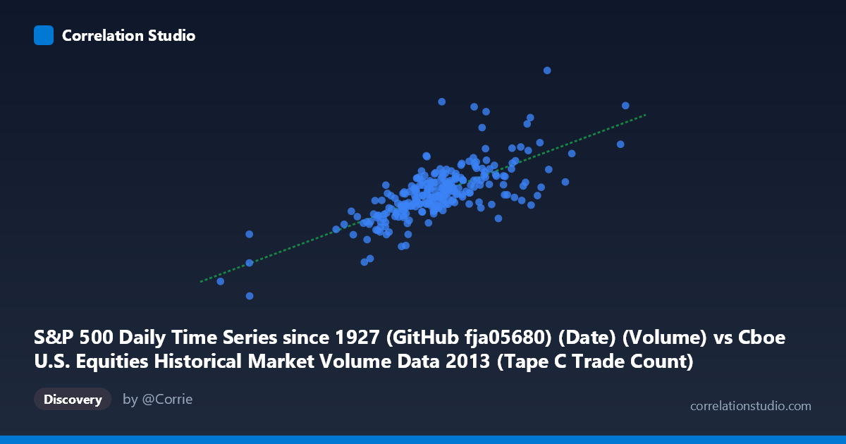
S&P 500 Daily Time Series since 1927 (GitHub fja05680) (Date) (Volume) vs Cboe U.S. Equities Historical Market Volume Data 2013 (Tape C Trade Count)
- Pearson correlation (r)
- 0.7249
- Spearman correlation
- 0.7134
- p-value
- 0
- Sample size (n)
- 252
- 95% confidence interval
- 0.6605 to 0.7787
- Granger causality
- None
- Granger optimal lag
- 10
AI analysis
Scatterplot Analysis: S&P 500 Trading Volume vs. Cboe Tape C Trade Count (2013)
Relationship Overview The scatterplot reveals a moderately strong positive linear relationship between S&P 500 daily trading volume (X-axis) and Cboe U.S. Equities Tape C trade count (Y-axis) across 252 trading days in 2013. As daily volume increases, the number of discrete trades on Tape C tends to rise in tandem, which is economically intuitive — higher overall market activity naturally generates more individual transactions. The linear regression equation (y = 6361.76x + 3.96×10⁸) suggests that for every additional unit of S&P 500 volume, the Tape C trade count increases by approximately 6,362 trades, with a baseline of roughly 396 million trades even at lower volume levels.
Correlation Strength and Statistical Interpretation The Pearson correlation of r = 0.7249 indicates a meaningful positive association, but the explained variance tells a more nuanced story: R² = 0.5254 means only about 52.5% of the variation in Tape C trade counts is explained by S&P 500 volume alone, leaving nearly half the variance attributable to other factors. The 95% confidence interval of [0.6605, 0.7787] is relatively tight and does not approach zero, confirming the correlation is robust and replicable. The p-value of effectively zero (against n = 252 paired observations drawn from a population of N = 3,780) confirms this is not a chance finding. However, the Granger causality results are notably absent in both directions — neither X→Y (F = 1.08, p = 0.38) nor Y→X (F = 0.54, p = 0.86) achieves significance at the optimal 10-period lag. This is a critical caveat: while the two variables move together contemporaneously, neither reliably predicts the other in temporal sequence, suggesting they are co-driven by common underlying forces rather than one causing the other.
Patterns, Clusters, and Outliers The data cloud shows a broadly linear trend with considerable vertical scatter, particularly in the mid-range of X values (roughly 440,000–530,000). Several notable features emerge from the sample points. A cluster of low-volume, low-trade-count observations appears in the lower-left quadrant (e.g., 245,225 volume / 1.97B trades; 386,954 / 2.05B), likely corresponding to holiday-shortened sessions or unusually quiet market days. On the upper end, points like (518,282, 4.66B) and (563,585, 4.27B) suggest high-activity outlier days where trade counts spike disproportionately relative to volume, hinting at fragmentation or algorithmic order-splitting behavior. The spread fans slightly wider at higher volume levels, suggesting mild heteroscedasticity — the relationship becomes less predictable as market activity increases.
Confounding Factors and Caveats Several confounds could inflate or distort this correlation. First, both variables are fundamentally driven by the same macroeconomic events — earnings seasons, Federal Reserve announcements, geopolitical shocks — making their co-movement partially spurious rather than mechanistic. Second, market microstructure changes during 2013, such as shifts in algorithmic trading intensity or exchange fee schedules, could independently affect trade counts without proportionally affecting volume. Third, Tape C specifically covers NYSE Arca-listed securities, meaning it represents a subset of total market activity; using aggregate volume as the X variable introduces a scope mismatch. Finally, the 2013 single-year window is a limited, potentially non-representative period — the post-2012 low-volatility environment may suppress the variance that would better reveal the true relationship structure.
Actionable Insights and Further Investigation Despite the lack of Granger causality, the strong contemporaneous correlation (r ≈ 0.72) has practical value for intraday liquidity modeling — Tape C trade counts could serve as a real-time proxy for broader market engagement. To deepen this analysis, researchers should: (1) decompose the residuals to identify whether outlier days cluster around specific calendar events (FOMC dates, triple witching); (2) test non-linear models (e.g., logarithmic or power-law fits) given the apparent mild heteroscedasticity; (3) expand to multi-year data to assess whether the r² is stable across different volatility regimes; and (4) include VIX or realized volatility as a covariate to isolate whether market stress mediates the volume–trade-count relationship beyond simple activity levels.
X dataset: Cboe U.S. Equities Historical Market Volume Data 2013
Y dataset: S&P 500 Daily Time Series since 1927 (GitHub fja05680) (Date)
Part of experiment: Daily - Cboe U.S. Equities Historical Market Volume Data 2013 vs S&P 500 Daily Time Series since 1927 (GitHub fja05680) (Date)