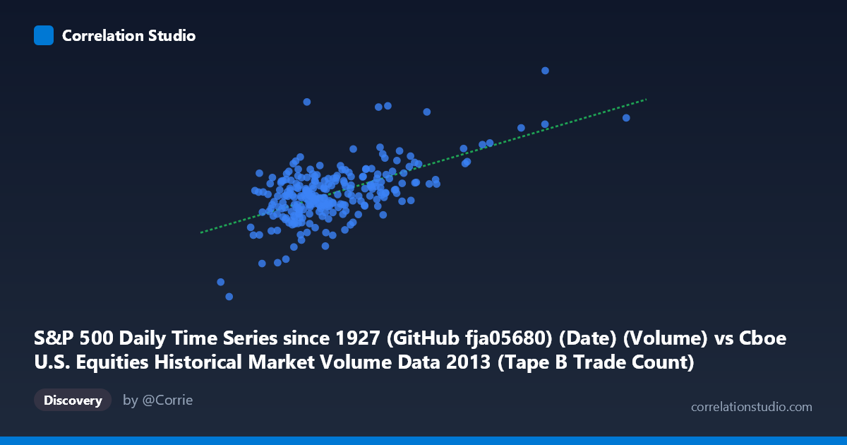
S&P 500 Daily Time Series since 1927 (GitHub fja05680) (Date) (Volume) vs Cboe U.S. Equities Historical Market Volume Data 2013 (Tape B Trade Count)
- Pearson correlation (r)
- 0.5997
- Spearman correlation
- 0.4588
- p-value
- 0
- Sample size (n)
- 252
- 95% confidence interval
- 0.5142 to 0.6734
- Granger causality
- None
- Granger optimal lag
- 10
AI analysis
Analysis: S&P 500 Daily Volume vs. Cboe Tape B Trade Count (2013)
Relationship Overview The scatterplot reveals a moderate positive relationship between S&P 500 daily trading volume and Cboe Tape B trade counts across 252 trading days in 2013. As overall market volume increases, Tape B trade counts tend to rise correspondingly, which is intuitively logical — higher market-wide activity generally propagates across exchange tapes and venues simultaneously. The linear regression equation (y = 7,340.57x + 2.08×10⁹) suggests that for every unit increase in S&P 500 volume, Tape B trade count increases by approximately 7,341 trades, with a substantial baseline intercept reflecting the persistent underlying trade flow independent of volume fluctuations.
Correlation Strength and Statistical Significance The Pearson correlation of r = 0.600 indicates a moderate positive association, but the explained variance (r² = 0.360) tells a more sobering story: only 36% of the variance in Tape B trade counts is attributable to S&P 500 volume. The remaining 64% is driven by other factors entirely. The 95% confidence interval [0.514, 0.673] is reasonably tight given n = 252, and the p-value of effectively zero confirms the relationship is statistically robust and not a sampling artifact. However, the Granger causality results are striking in their absence — neither direction (X→Y: F = 0.51, p = 0.88; Y→X: F = 0.59, p = 0.82) achieves significance at any conventional threshold, even with an optimal lag of 10 periods. This means that despite the contemporaneous correlation, neither variable reliably predicts the other temporally, ruling out a simple leading-indicator relationship.
Notable Patterns and Outliers The scatterplot displays considerable vertical dispersion at most X-values, particularly in the mid-range volume zone (150,000–200,000), where Tape B trade counts vary widely from roughly 2.3 billion to 4.3 billion — a near-doubling range for similar volume levels. Several notable outliers are visible: a cluster of high-volume, high-trade-count days (X 280,000, particularly the point near 327,000 volume with ~4.66 billion trades) sits distinctly apart from the main body, potentially representing options expiration days or macro shock events. Conversely, points like (168,572; 2.31 billion) and (136,643; 2.05 billion) appear as low-trade-count anomalies that pull against the regression line, suggesting days where volume occurred in large block sizes rather than high-frequency small orders.
Confounding Factors and Caveats Several important caveats apply. First, Tape B specifically covers NYSE American (AMEX) and regional exchange securities, meaning it doesn't map cleanly onto S&P 500 constituents, which are predominantly Tape A securities — this structural mismatch likely suppresses the true correlation and introduces noise. Second, both variables are subject to shared macroeconomic drivers (VIX spikes, Fed announcements, earnings seasons) that create spurious synchrony without causal linkage — a classic omitted variable problem. Third, the 2013 sample period is historically specific: post-crisis market structure with recovering volumes, HFT proliferation, and specific regulatory environment may limit generalizability. The large population size (N = 3,780 referenced) versus the sample (n = 252) also warrants attention regarding how the sample was constructed.
Actionable Insights and Further Investigation Practitioners should not use S&P 500 volume as a predictive signal for Tape B trade activity — the Granger results make this clear despite the surface-level correlation. More productive next steps would include: (1) decomposing by market regime (low-VIX vs. high-VIX periods) to test whether the correlation strengthens during stress events; (2) controlling for time-of-year effects such as quarterly expiration cycles and holiday-adjacent low-volume days, which likely explain several outlier clusters; (3) testing Tape A and Tape C volumes separately against S&P 500 volume to find structurally appropriate comparisons; and (4) examining trade size distributions rather than count alone, since the weak explanatory power (64% unexplained variance) strongly suggests that order fragmentation behavior — not raw volume — is the missing variable driving Tape B trade count independently of aggregate market activity.
X dataset: Cboe U.S. Equities Historical Market Volume Data 2013
Y dataset: S&P 500 Daily Time Series since 1927 (GitHub fja05680) (Date)
Part of experiment: Daily - Cboe U.S. Equities Historical Market Volume Data 2013 vs S&P 500 Daily Time Series since 1927 (GitHub fja05680) (Date)