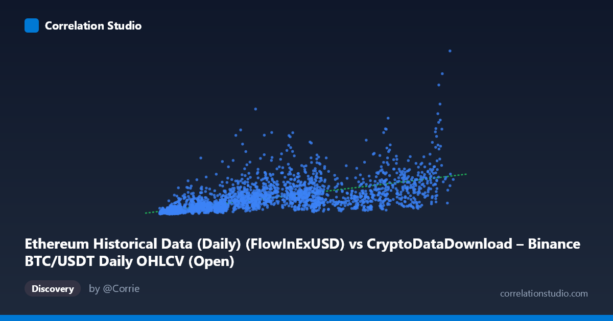
Ethereum Historical Data (Daily) (FlowInExUSD) vs CryptoDataDownload – Binance BTC/USDT Daily OHLCV (Open)
- Pearson correlation (r)
- 0.6577
- Spearman correlation
- 0.8179
- p-value
- 0
- Sample size (n)
- 3191
- 95% confidence interval
- 0.6375 to 0.6769
- Granger causality
- Y → X
- Granger optimal lag
- 10
AI analysis
Analysis of the X–Y Relationship
1. What the visualization reveals
The scatterplot shows a positive, moderately strong association between the X variable (labeled as Ethereum flow-in, though metadata suggests it may actually be a mislabeled BTC-related field) and Y (Bitcoin's daily opening price). As X increases, Y tends to rise as well, but the relationship is not tight — points fan out considerably, especially at low-to-mid X values, where Y ranges from tens of millions to over a billion. This spread narrows somewhat at higher X values, suggesting the relationship may flatten or saturate rather than continue linearly.
2. Strength, direction, and statistical confidence
The Pearson correlation (r = 0.658) indicates a moderate-to-strong positive linear relationship, with r² = 0.4325 meaning only about 43% of the variance in Y is explained by X — leaving more than half unexplained by this single variable. The 95% CI [0.6375, 0.6769] is tight given the large sample (n=3,191), and the p-value of ~0 confirms the correlation is highly statistically significant and not due to chance. However, statistical significance here reflects sample size more than practical predictive strength — r² of 0.43 is moderate, not dominant.
The Granger causality results add an important directional insight: Y Granger-causes X, not the other way around (Y→X: F=2.60, p=0.0038 vs X→Y: F=1.51, p=0.128). This means past values of Y (BTC price) have predictive power for future values of X, but not vice versa. This is a meaningful finding — it suggests X is a lagging or responsive variable relative to Y, rather than a leading indicator. Practically, this undercuts any assumption that X could be used to forecast Y; the causal (predictive) direction appears reversed from what a naive reading of "X causes Y" might imply.
3. Notable patterns and non-linear features
The note that Spearman's ρ exceeds Pearson's r is a strong signal of non-linearity — the rank-based correlation captures monotonic structure better than the linear fit does. This is consistent with the visual pattern: variance in Y appears to grow with X (heteroscedasticity), and there may be diminishing returns at high X (a logarithmic or power-law shape) rather than a straight line. Several sample points show extreme Y values (1.3–1.8 billion) at moderate X (~40,000–70,000), representing outliers or a volatile sub-cluster — possibly tied to specific market events or dates where BTC price spiked independent of the X metric. These outliers likely inflate the residual scatter and pull down the linear r².
4. Confounding factors and caveats
Several caveats are critical here. First, the metadata is inconsistent/confusing — X is labeled as an Ethereum flow metric but tied to a Binance BTC OHLCV dataset, and Y (labeled Ethereum Open) is actually BTC/USDT Open price. This suggests possible data-pipeline mislabeling, which should be resolved before drawing market conclusions. Second, both series span 2017–2026, a period covering multiple bull/bear cycles, meaning the correlation is likely driven by shared macro trends (overall crypto market growth, BTC/ETH co-movement) rather than a direct causal mechanism. Third, daily financial time series are typically non-stationary and autocorrelated, which can inflate both correlation and Granger causality statistics — proper differencing/log-transformation and stationarity testing (ADF/KPSS) should precede causal interpretation. Finally, the "N=3,212 vs n=3,191" gap indicates ~21 missing/unpaired points, which could introduce selection bias if missingness correlates with volatility events.
5. Actionable insights
- Clarify variable labeling before further analysis — confirm whether X and Y are correctly sourced and not artifacts of a data-merge error. - Test non-linear models (log-log, polynomial, or spline regression) given the Spearman/Pearson divergence; a log transform of both variables may substantially improve fit and stabilize variance. - Investigate the Y→X Granger direction further with impulse-response analysis to quantify lag effects and economic significance, not just statistical significance. - Segment by market regime (bull/bear/sideways) since pooled correlation across a full multi-year cycle can mask regime-dependent relationship changes. - Check stationarity and consider differencing the series before trusting Granger causality results, as spurious causality is common in trending financial data.
X dataset: CryptoDataDownload – Binance BTC/USDT Daily OHLCV
Y dataset: Ethereum Historical Data (Daily)
Part of experiment: Bitcoin - CryptoDataDownload – Binance BTC/USDT Daily OHLCV vs Ethereum Historical Data (Daily)