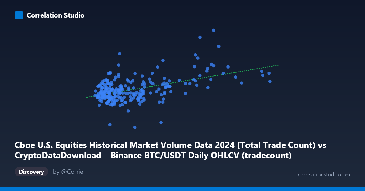
Cboe U.S. Equities Historical Market Volume Data 2024 (Total Trade Count) vs CryptoDataDownload – Binance BTC/USDT Daily OHLCV (tradecount)
- Pearson correlation (r)
- 0.5022
- Spearman correlation
- 0.3429
- p-value
- 0
- Sample size (n)
- 252
- 95% confidence interval
- 0.4037 to 0.5892
- Granger causality
- None
- Granger optimal lag
- 10
AI analysis
Analysis: Cboe U.S. Equities Trade Count vs. Binance BTC/USDT Trade Count (2024)
1. What the Visualization Reveals
The scatterplot shows a positive but noisy relationship between two trade-count metrics from entirely different markets: Cboe U.S. equities trade counts (X) and Binance BTC/USDT trade counts (Y). The bulk of observations cluster tightly in the lower-left region (X roughly 900K–5.5M, Y roughly 3.4M–4.7M), while a handful of points extend far to the right (X 7.5M, up to 12M), representing days of unusually heavy equities trading. This creates a classic "comet" or "wedge" shape rather than a clean linear cloud, with most of the correlation signal being driven by the scatter's general upward drift rather than a tight linear band.
2. Strength, Direction, and Statistical Confidence
The correlation coefficient (r = 0.502) indicates a moderate positive relationship, but r² = 0.252 means only about 25% of the variance in Binance trade counts is explained by Cboe equity trade counts — leaving 75% driven by other factors. The 95% CI [0.404, 0.589] is reasonably tight given n=252, and the p-value (effectively 0) confirms the correlation is statistically significant and not due to chance. However, statistical significance here should not be conflated with practical predictive power — an r² of 0.25 is modest. Critically, the Granger causality tests show no significant predictive direction in either direction (X→Y: p=0.587; Y→X: p=0.749), meaning that despite the contemporaneous correlation, neither series helps forecast the other's future values based on its own lagged history. This strongly suggests the relationship is either coincidental, driven by a shared external factor, or purely contemporaneous rather than a lead-lag dynamic.
3. Notable Patterns and Outliers
Several high-leverage points stand out: (8250511, 4535947), (8066322, 4169506), (9048605, 4812478), and (12012364-range point) sit far outside the main cluster on the X-axis, likely corresponding to specific high-volume equity trading days (e.g., quarterly rebalancing, options expiration, or major market events like a Fed announcement). One notable Y-axis outlier is (7568497, 6425683) — a day with both elevated equities activity and an unusually high Bitcoin trade count, sitting well above the regression line. Another mild outlier is (3421549, 2387080), which falls well below the main band on the Y-axis. These high-leverage points, especially the four with X 7.5M, likely have outsized influence on the regression slope (0.118) and the r² value — the relationship in the dense main cluster looks considerably weaker and more scattered than the overall statistic suggests.
4. Confounding Factors and Caveats
Both time series are essentially daily activity/liquidity proxies that could be correlated simply because they both spike on days of general macro volatility (CPI releases, FOMC meetings, geopolitical shocks) — a classic shared confounder problem rather than a direct causal link between equities and crypto trading. Additionally, trade count is a mechanical/structural metric (affected by algo trading, market maker activity, exchange fee schedules, and API-driven order flow) rather than a pure economic signal, so comparing tradecounts across two structurally different market types (regulated equities exchanges vs. a crypto exchange) may not be an apples-to-apples comparison. The small number of extreme X-axis outliers also raises concern about leverage effects: removing those 4-5 points could substantially change r and r². Finally, 252 paired daily points from a single calendar year is a limited sample for capturing structural relationships that may shift with market regime (bull vs. bear crypto markets, changing equity market structure).
5. Suggestions for Further Investigation
1. Robustness check: Re-run the correlation after removing/winsorizing the 4-5 high-leverage X outliers to see if r² holds or collapses — this will clarify whether the relationship is driven by a few extreme days. 2. Control for a common driver: Introduce a volatility index (VIX) or major macro event calendar as a covariate to test whether the correlation is spurious/confounded by shared market-wide volatility. 3. Non-linear/log transforms: Given the wedge-shaped scatter and heavy right-skew in X, try log-transforming both variables to check for a more stable, less leverage-sensitive relationship. 4. Extend the causality analysis: Test Granger causality using volume/dollar value instead of trade count, and explore contemporaneous (lag-0) relationships more rigorously (e.g., cross-correlation function) since the current lag-10 test found nothing but same-day correlation is still significant. 5. Segment by regime: Split the year into risk-on/risk-off periods or crypto bull/bear phases to see if the correlation strengthens or weakens during specific market conditions, which would be more actionable than a single blended annual r².
X dataset: CryptoDataDownload – Binance BTC/USDT Daily OHLCV
Y dataset: Cboe U.S. Equities Historical Market Volume Data 2024
Part of experiment: Bitcoin - CryptoDataDownload – Binance BTC/USDT Daily OHLCV vs Cboe U.S. Equities Historical Market Volume Data 2024