Ethereum Historical Price Data (AssetCompletionTime) vs CryptoDataDownload – Binance BTC/USDT Daily OHLCV (Low)
- Pearson correlation (r)
- 0.8552
- Spearman correlation
- 0.89
- p-value
- 0
- Sample size (n)
- 3191
- 95% confidence interval
- 0.8456 to 0.8642
- Granger causality
- None
- Granger optimal lag
- 10
- Time coverage
- 2017-08-17 to 2026-05-20
AI analysis
Analysis of BTC/USDT–Ethereum Price Relationship
Note on data labeling: The axis labels appear mismatched with the actual sample data — the X column is described as "Ethereum Historical Price Data (AssetCompletionTime)" but values (2,817–123,084) are far too low to be ETH prices in this era and look like a completion-time or index metric, while Y values (~1.6–1.78 billion) are clearly not BTC/USDT low prices. The Y values appear to be Unix timestamps (corresponding to 2017–2026, consistent with the stated time coverage) rather than a price series. This analysis proceeds based on the statistical relationship as given, but the variable identities should be verified before drawing market conclusions.
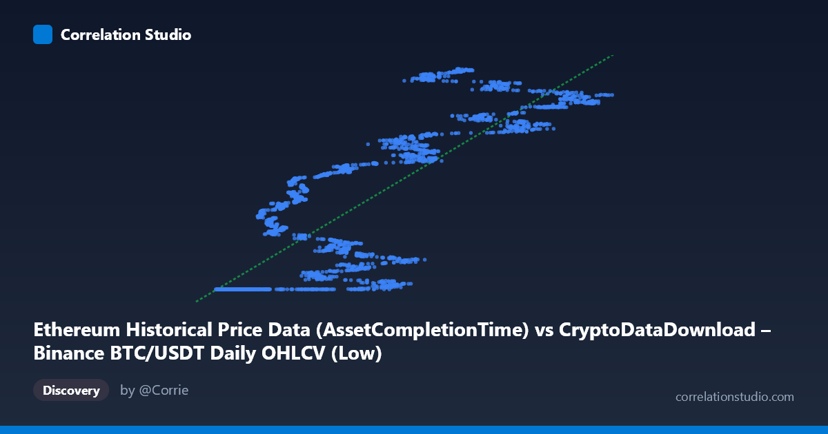
1. Overall Relationship The scatterplot shows a strong, positive, and highly non-linear (piecewise) relationship. A large cluster of points sits at a nearly constant Y value (~1,614,335,225–1,614,335,700) across a wide range of X (roughly 3,700–35,000), forming a flat "floor." Beyond X≈35,000, Y rises steeply and continuously with X, reaching the range maximum (~1.78 billion) by X≈80,000–110,000. This creates a hockey-stick or threshold pattern rather than a simple straight-line trend.
2. Strength, Direction, and Statistical Confidence The linear correlation coefficient (r = 0.855) indicates a strong positive association, with r² = 0.731 meaning the linear model explains about 73% of the variance in Y — leaving roughly 27% unexplained, likely due to the non-linear floor/ramp structure described above. The 95% CI [0.846, 0.864] is tight, and p ≈ 0 confirms this correlation is highly unlikely to be due to chance given the large sample (n = 3,191). However, correlation strength should not be read as causation: the Granger causality tests show no significant predictive direction in either direction (X→Y: p = 0.357; Y→X: p = 0.190) at the optimal lag of 10 periods. This means neither series reliably helps forecast the other's future values based on past values — the strong contemporaneous correlation likely reflects a shared underlying driver (e.g., a common time trend or index) rather than one variable causing or leading the other.
3. Notable Patterns and Features - Flat cluster/plateau: A dense set of points where Y is essentially constant (~1,614,335,xxx) despite X varying from ~3,700 to ~35,000 — suggesting a floor, censoring effect, or an early period where Y was pinned to a minimum/baseline value. - Steep ramp: Above X≈35,000, Y increases sharply and near-linearly with X, suggesting the relationship "activates" only past a threshold. - Two regimes: The data essentially behaves as two distinct sub-populations — a flat regime and a rising regime — which explains why a single linear fit only captures 73% of variance despite a visually strong trend in the upper range. - No obvious extreme outliers were noted beyond this two-regime structure; the pattern is systematic rather than driven by isolated anomalies.
4. Confounding Factors and Caveats - Likely temporal confounding: If Y is actually a timestamp or time-indexed value, the "correlation" may simply reflect that both series evolve over the same calendar period, not a genuine causal or economic relationship. - Non-linearity misrepresented by r²: Since the relationship is piecewise (flat then rising), the linear r² of 0.731 understates the true explanatory power of a segmented or non-linear model. - Data labeling inconsistency: As noted, the described axis variables (ETH price vs. BTC/USDT low) don't match the actual value ranges — this should be resolved before any market interpretation is finalized. - Autocorrelation in time series: Both variables likely have strong internal autocorrelation (trends over time), which can inflate correlation coefficients between two unrelated but co-trending series (spurious regression risk).
5. Suggested Next Steps - Verify variable definitions/units before proceeding — confirm whether Y is truly a price or a timestamp artifact from data processing. - Fit a segmented/non-linear model (e.g., piecewise regression or spline) to better capture the plateau-then-ramp structure and improve on the 73% linear R². - Difference or detrend the series and re-test correlation/Granger causality on returns rather than levels, to check whether the relationship holds independent of shared time trends. - Investigate the threshold point (~X=35,000) driving the regime shift — this could correspond to a meaningful market event, data collection change, or structural break worth explaining domain-wise.
X dataset: CryptoDataDownload – Binance BTC/USDT Daily OHLCV
Y dataset: Ethereum Historical Price Data
Part of experiment: Bitcoin - CryptoDataDownload – Binance BTC/USDT Daily OHLCV vs Ethereum Historical Price Data