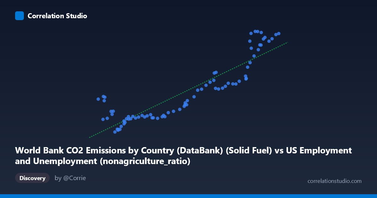
World Bank CO2 Emissions by Country (DataBank) (Solid Fuel) vs US Employment and Unemployment (nonagriculture_ratio)
- Pearson correlation (r)
- 0.8938
- Spearman correlation
- 0.8706
- p-value
- 0
- Sample size (n)
- 80
- 95% confidence interval
- 0.8387 to 0.9307
- Granger causality
- None
- Granger optimal lag
- 10
AI analysis
Scatterplot Analysis: Solid Fuel CO2 Emissions vs. US Non-Agricultural Employment Ratio
1. Overall Relationship The scatterplot reveals a strong positive relationship between World Bank solid fuel CO2 emissions and the US non-agricultural employment ratio, spanning eight decades from 1941 to 2020. As solid fuel CO2 emissions increase, the non-agricultural employment ratio rises in a broadly linear fashion, following the regression line y = 0.163x + 2535.7. However, the scatter around this line is notably uneven, with tighter clustering at lower emission values and considerably more dispersion at higher values (roughly above 120,000 units), suggesting the relationship becomes less predictable at higher emission levels and that a simple linear model may not fully capture the dynamics across the full historical range.
2. Correlation Strength and Statistical Significance The Pearson correlation of r = 0.894 indicates a strong positive association, and the R² of 0.799 means approximately 79.9% of the variance in the non-agricultural employment ratio is statistically explained by solid fuel CO2 emissions. The 95% confidence interval for r of [0.839, 0.931] is relatively narrow, confirming this is a robust estimate unlikely to be a statistical artifact, and the p-value of effectively zero confirms the association is highly significant given n = 80 paired observations. That said, the remaining ~20% of unexplained variance is non-trivial and likely reflects meaningful real-world complexity. Critically, Granger causality tests find no significant predictive directionality in either direction (X→Y: F = 1.06, p = 0.41; Y→X: F = 1.11, p = 0.37, optimal lag = 10 periods). This is an important qualification: despite the strong correlation, neither variable reliably predicts the future trajectory of the other in a temporal sense, cautioning against any causal interpretation.
3. Notable Patterns, Clusters, and Outliers Several structural features stand out in the data. The lower-emission range (roughly 41,000–90,000) forms a relatively tight cluster with modest non-agricultural ratios, consistent with the post-WWII through mid-20th century industrial period. A second, more dispersed cluster appears in the upper range (130,000–155,000 emissions), where y-values fan out considerably — for instance, points near x ≈ 140,000–145,000 span y-values from roughly 25,000 to over 31,000, indicating high variability in labor market composition at peak emission periods. Several points near the lower-left (e.g., x ≈ 41,250–46,930 paired with relatively high y-values of 12,266–17,183) appear as potential outliers or structural breaks, possibly reflecting wartime or early post-war labor anomalies where non-agricultural employment was elevated despite lower industrial fuel use. These leverage points could disproportionately influence the regression slope and warrant individual examination.
4. Confounding Factors and Interpretive Caveats The most significant caveat is that both variables are strongly driven by a common third factor: long-run economic and population growth over the 1941–2020 period. Both solid fuel emissions and the non-agricultural workforce share a near-monotonic upward secular trend driven by GDP expansion, industrialization, and demographic growth, meaning much of the observed correlation is a spurious time-trend artifact rather than a direct mechanistic link. Additionally, the dataset description itself reveals a probable data provenance mismatch: X is labeled as coming from a "US Employment" dataset while Y is labeled as coming from a "CO2 Emissions" dataset, suggesting these columns may have been joined across datasets with differing original contexts, raising data integrity concerns. Structural breaks — such as the 1970s oil crises, the 2008 financial crisis, or the post-2000 shift away from coal in the US energy mix — could create regime-dependent relationships that a single linear model masks entirely.
5. Actionable Insights and Further Investigation Given the absence of Granger causality, this correlation should not be used for forecasting or policy levers without substantially deeper modeling. Recommended next steps include: (1) detrending both series (e.g., first-differencing or HP filtering) to remove shared secular trends and test whether a residual correlation persists; (2) segmenting the analysis by decade to detect whether the correlation strengthens, weakens, or reverses across different economic regimes; (3) introducing explicit controls such as GDP, population, energy mix composition, and labor force participation rates to isolate any partial correlation net of confounders; (4) investigating the anomalous low-emission/high-employment-ratio observations individually, as they may represent historically important structural breaks; and (5) verifying the dataset join logic to ensure that the CO2 and employment columns correspond to the same country-year observations, as the cross-dataset labeling raises legitimate data quality questions that could invalidate the current analysis.
X dataset: US Employment and Unemployment
Y dataset: World Bank CO2 Emissions by Country (DataBank)
Part of experiment: Yearly - US Employment and Unemployment vs World Bank CO2 Emissions by Country (DataBank)