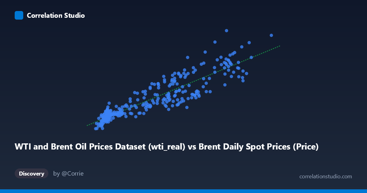
WTI and Brent Oil Prices Dataset (wti_real) vs Brent Daily Spot Prices (Price)
- Pearson correlation (r)
- 0.9032
- Spearman correlation
- 0.9219
- p-value
- 0
- Sample size (n)
- 295
- 95% confidence interval
- 0.8797 to 0.9222
- Granger causality
- None
- Granger optimal lag
- 4
AI analysis
Analysis: WTI Real Prices vs. Brent Nominal Prices (1987–2026)
1. Overall Relationship The scatterplot reveals a strong, positive, and largely linear relationship between Europe Brent crude oil spot prices (nominal, X-axis) and CPI-adjusted WTI crude oil prices (real, Y-axis). As Brent nominal prices rise, real WTI prices rise in near-lockstep, which is consistent with the well-established co-movement of global crude oil benchmarks. The regression line (y = 0.974x + 26.64) indicates that for every additional dollar in Brent nominal price, real WTI prices increase by approximately $0.97, while the intercept of ~$26.64 reflects the persistent baseline premium that CPI inflation adjustment adds to WTI prices across the time series — a conceptually sensible artifact of comparing nominal Brent to inflation-deflated WTI.
2. Correlation Strength and Statistical Significance The correlation of r = 0.903 is exceptionally strong, and the R² of 0.816 means that approximately 81.6% of the variance in real WTI prices is explained by nominal Brent prices alone — a remarkably high figure for a nearly four-decade economic time series. The 95% confidence interval of [0.880, 0.922] is narrow, indicating high precision in this estimate, and the p-value of ~0 confirms the relationship is not a statistical artifact. However, the Granger causality results are notably non-significant in both directions (X→Y: F=1.32, p=0.26; Y→X: F=1.14, p=0.34), meaning neither series reliably predicts the other temporally at the tested lag of 4 periods. This is an important nuance: the two series move together contemporaneously, but neither leads the other in a predictive sense, suggesting they respond to the same underlying market forces rather than one driving the other.
3. Notable Patterns, Clusters, and Outliers The scatterplot exhibits a clear bimodal clustering structure: a dense cluster of low-price observations concentrated in the roughly $10–$30 Brent / $25–$65 WTI range, corresponding to the pre-2000s and post-2014 oil price collapse periods, and a more dispersed upper cluster spanning $60–$140 Brent / $70–$170 WTI, likely reflecting the 2005–2008 and 2010–2014 commodity supercycles. A handful of points in the upper-right quadrant (e.g., ~119 Brent / ~168 WTI) appear as potential high-leverage outliers, possibly corresponding to the 2008 price spike or post-COVID 2022 surge. These extreme observations could be disproportionately influencing the slope and R². The lower cluster also shows somewhat higher vertical scatter relative to the regression line, suggesting the inflation adjustment introduces more noise at low nominal price levels.
4. Confounding Factors and Caveats Several important caveats qualify this correlation. First, the comparison is conceptually asymmetric — one variable is nominal (Brent) and the other is CPI-adjusted (WTI) — meaning part of the explained variance may simply reflect shared nominal price inflation rather than a true structural relationship. The ~$26 intercept likely embeds decades of cumulative inflation. Second, sampling every 5th observation (n=295 from N=483) and the use of monthly-or-lower-frequency aggregation may obscure short-term divergences between the two benchmarks, such as the WTI-Brent spread that widened significantly during 2011–2013 due to U.S. pipeline bottlenecks. Third, structural breaks across the 39-year period — OPEC policy shifts, U.S. shale revolution, COVID-19 demand collapse — likely mean the relationship is not stationary, and a single linear model may be overfitting stable regime periods while masking regime-specific dynamics.
5. Actionable Insights and Further Investigation Given the high contemporaneous correlation but absent Granger causality, analysts should treat these two series as joint indicators of a common latent factor (global oil market conditions) rather than using one to forecast the other. Practically, this means hedging or pricing models should incorporate both benchmarks against shared drivers (e.g., global demand proxies, USD index, geopolitical risk indices) rather than substituting one for the other. For further investigation, it would be valuable to: (a) convert both series to the same real or nominal basis to eliminate the inflation-induced intercept artifact; (b) fit a piecewise or regime-switching model to test whether the slope and intercept differ across oil market eras; (c) explicitly model the WTI-Brent spread as a dependent variable to identify periods of benchmark divergence; and (d) test Granger causality at shorter lags (1–2 periods) and on first-differenced data to better capture high-frequency predictive dynamics between the two markets.
X dataset: Brent Daily Spot Prices
Y dataset: WTI and Brent Oil Prices Dataset
Part of experiment: Daily - Brent Daily Spot Prices vs WTI and Brent Oil Prices Dataset