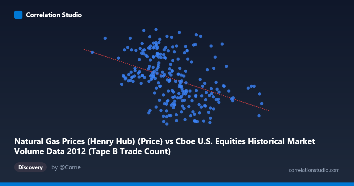
Natural Gas Prices (Henry Hub) (Price) vs Cboe U.S. Equities Historical Market Volume Data 2012 (Tape B Trade Count)
- Pearson correlation (r)
- -0.4093
- Spearman correlation
- -0.4551
- p-value
- 0
- Sample size (n)
- 250
- 95% confidence interval
- -0.5076 to -0.3004
- Granger causality
- None
- Granger optimal lag
- 1
AI analysis
Analysis: Natural Gas Prices vs. Cboe Equity Market Trade Count (2012)
Relationship Overview
The scatterplot reveals a moderate negative relationship between U.S. equity market trade volume (Tape B Trade Count, on the X-axis) and Henry Hub natural gas spot prices (Y-axis) across the 2012 trading year. As equity market activity increases, natural gas prices tend to decline, and vice versa. The linear regression equation (y = -4.95E-06x + 3.618) quantifies this inverse slope, suggesting that for every increase of roughly 200,000 trades, the model predicts approximately a one-cent decline in natural gas prices. The data spans a meaningful range — trade counts from ~63,000 to ~298,000 and gas prices from $1.82 to $3.77 — capturing substantial variation across both dimensions during a year notable for historically low natural gas prices and evolving equity market structure.
Correlation Strength and Statistical Significance
The correlation coefficient of r = -0.409 indicates a moderate negative association, but the explanatory power is notably limited: r² = 0.167, meaning only 16.7% of the variance in natural gas prices is accounted for by equity trade volume. The remaining ~83% of price variation is driven by factors entirely outside this model. The 95% confidence interval of [-0.508, -0.300] is meaningfully negative throughout and does not cross zero, lending credibility to the directional finding. The p-value of 1.63E-11 is highly statistically significant given n = 250 paired observations drawn from a population of 3,750, making it very unlikely this correlation arose by chance. However, statistical significance here should not be conflated with practical significance or causation — the modest r² cautions strongly against over-interpretation. Critically, Granger causality testing finds no significant predictive direction in either direction (X→Y: F = 0.757, p = 0.385; Y→X: F = 1.952, p = 0.164), meaning neither variable temporally predicts the other at a one-period lag. This firmly rules out a straightforward leading-indicator or causal mechanism between equity trading activity and natural gas pricing.
Notable Patterns, Clusters, and Outliers
Several features stand out in the sample points. There is a visible cluster of moderate trade counts (roughly 140,000–200,000) associated with a wide spread of gas prices ($2.20–$3.65), suggesting high price variability even within a narrow band of trading activity — consistent with the low r². At higher trade counts (220,000), gas prices tend to compress toward the lower range ($1.82–$2.61), reinforcing the negative trend but with notable scatter. A few points warrant attention as potential outliers: (295,121; 2.44) represents an unusually high trade count with a mid-range gas price, while (207,237; 3.66) and (173,304; 3.61) show elevated gas prices paired with moderate trade activity. The lower-left region (low trade counts, moderate-to-high prices) also shows meaningful dispersion. There is no strong evidence of a non-linear pattern from the sample, though the wide vertical scatter at mid-range X values hints at heteroscedasticity that a simple linear model may not fully capture.
Confounding Factors and Caveats
This correlation almost certainly reflects shared dependence on common macroeconomic drivers rather than any direct link between equity trading volume and natural gas prices. Both variables are heavily influenced by broader economic conditions, seasonal cycles, and market sentiment in 2012 — a year characterized by the U.S. shale gas boom driving historically suppressed natural gas prices and shifting equity market microstructure post-financial crisis. Seasonality is a major confounder: natural gas prices exhibit strong winter/summer patterns tied to heating and cooling demand, while equity volumes follow their own seasonal rhythms (e.g., lower summer volumes). The dataset label metadata also appears inverted (X-axis labeled from gas price dataset, Y-axis from equity dataset), which should be verified before drawing any directional conclusions. Additionally, using Tape B trade count specifically (regional exchanges) rather than total market volume introduces selection bias, as Tape B behavior may not represent aggregate market conditions. The one-period Granger lag tested may also be too short or too long to detect any delayed relationships.
Actionable Insights and Further Investigation
Given that only ~17% of variance is explained and no Granger causality is detected, practitioners should avoid using equity trade volume as a predictive signal for natural gas prices (or vice versa) in any trading or risk model without substantial additional validation. For further investigation, it would be valuable to: (1) decompose both series for seasonality before re-running correlation to isolate whether the relationship persists after removing shared seasonal trends; (2) test longer Granger lags (5, 10, or 22 trading days) to check for slower-moving predictive relationships; (3) introduce explicit confounders such as temperature data, crude oil prices, and broad market indices (S&P 500) into a multivariate regression to assess whether the negative correlation survives controls; and (4) examine sub-period correlations (Q1 vs. Q4) to determine whether the relationship is stable or driven by a specific regime within 2012. This analysis is best treated as exploratory — a prompt for deeper causal modeling rather than a standalone finding.
X dataset: Cboe U.S. Equities Historical Market Volume Data 2012
Y dataset: Natural Gas Prices (Henry Hub)
Part of experiment: Daily - Cboe U.S. Equities Historical Market Volume Data 2012 vs Natural Gas Prices (Henry Hub)