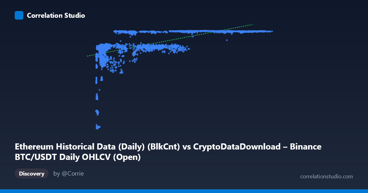
Ethereum Historical Data (Daily) (BlkCnt) vs CryptoDataDownload – Binance BTC/USDT Daily OHLCV (Open)
- Pearson correlation (r)
- 0.5723
- Spearman correlation
- 0.7299
- p-value
- 0
- Sample size (n)
- 3191
- 95% confidence interval
- 0.5485 to 0.5952
- Granger causality
- None
- Granger optimal lag
- 1
- Time coverage
- 2017-08-17 to 2026-05-20
AI analysis
Analysis: BTC Block Count vs. ETH Opening Price
1. What the Visualization Reveals
The scatterplot shows a clear non-linear, saturating relationship rather than a simple linear one. At low X values (roughly 3,000–15,000), Y climbs steeply from ~2,800 to ~6,400 — a dramatic rise packed into a narrow X range. Beyond X≈20,000, Y plateaus in a tight band between roughly 6,300 and 7,180, regardless of how far X extends (up to 124,000+). This produces a classic "hockey-stick" or logarithmic curve shape: rapid initial growth followed by a long, flat asymptote.
2. Strength, Direction, and Statistical Confidence
The Pearson correlation (r = 0.572, r² = 0.328) indicates a moderate positive linear association, but only 32.8% of Y's variance is explained by a straight-line fit to X — meaning linear correlation substantially understates the true relationship, since the pattern is curved rather than linear. The narrow 95% CI [0.549, 0.595] and p≈0 confirm this moderate correlation estimate is statistically robust and not due to chance, given the large sample (n=3,191). However, statistical significance here reflects sample size, not necessarily practical linear predictability. The note that Spearman ρ exceeds Pearson r reinforces that a monotonic but curved (log-like) relationship fits far better than a straight line. Critically, Granger causality tests show no predictive direction in either direction (X→Y: p=0.498; Y→X: p=0.792) — neither series helps forecast the other's future values based on past values. This strongly suggests the correlation is not causal in a time-series sense, but likely reflects both variables independently trending upward over the 2017–2026 period (a classic spurious correlation via shared temporal drift).
3. Notable Patterns and Outliers
The most striking feature is the early cluster of low-X, low-Y points (X < 10,000, Y < 6,500) — these represent early period data (likely 2017–2018) where both BTC block count and ETH price were low and rising together. Once X exceeds ~20,000–30,000, Y values compress into a narrow high band (6,300–7,180), creating a horizontal "ceiling" pattern with high scatter density but minimal vertical spread. This ceiling effect, rather than continued proportional growth, is the primary driver of the poor linear fit. No extreme outliers are apparent; the data forms a coherent curve rather than showing anomalous points.
4. Confounding Factors and Caveats
This is a cross-dataset time-series comparison — BTC block count (a network activity metric) versus ETH opening price (a market price metric) — from different underlying assets. Both variables likely share a common confounder: time itself, or more specifically, overall crypto market maturation, adoption growth, and secular price/activity inflation across the 2017–2026 window. Block count and price are both non-stationary series that trend upward over time, which mechanically inflates correlation without implying any functional relationship. Additionally, mismatched units (blocks vs. USD) and differing volatility regimes (e.g., ETH price crashes/rallies vs. steadily growing BTC block count) mean the relationship may be an artifact of two unrelated upward trends rather than genuine interaction.
5. Suggestions for Further Investigation
- Refit with a logarithmic or power model (Y ~ log(X)) given the clear saturation curve; this should substantially improve R² over the linear 32.8%. - Detrend or difference both series (e.g., use daily returns/changes instead of levels) to test whether correlation persists after removing shared time trends — this would clarify whether any genuine relationship exists beyond common drift. - Segment by time period (e.g., pre/post-2020) to check whether the relationship is stable or driven by a specific early-adoption era. - Given the null Granger causality result, avoid using one series to forecast the other; instead treat the correlation as descriptive/structural rather than predictive. - Consider whether a third variable (e.g., overall crypto market cap, adoption rate, or time index) better explains both series jointly.
X dataset: CryptoDataDownload – Binance BTC/USDT Daily OHLCV
Y dataset: Ethereum Historical Data (Daily)
Part of experiment: Bitcoin - CryptoDataDownload – Binance BTC/USDT Daily OHLCV vs Ethereum Historical Data (Daily)