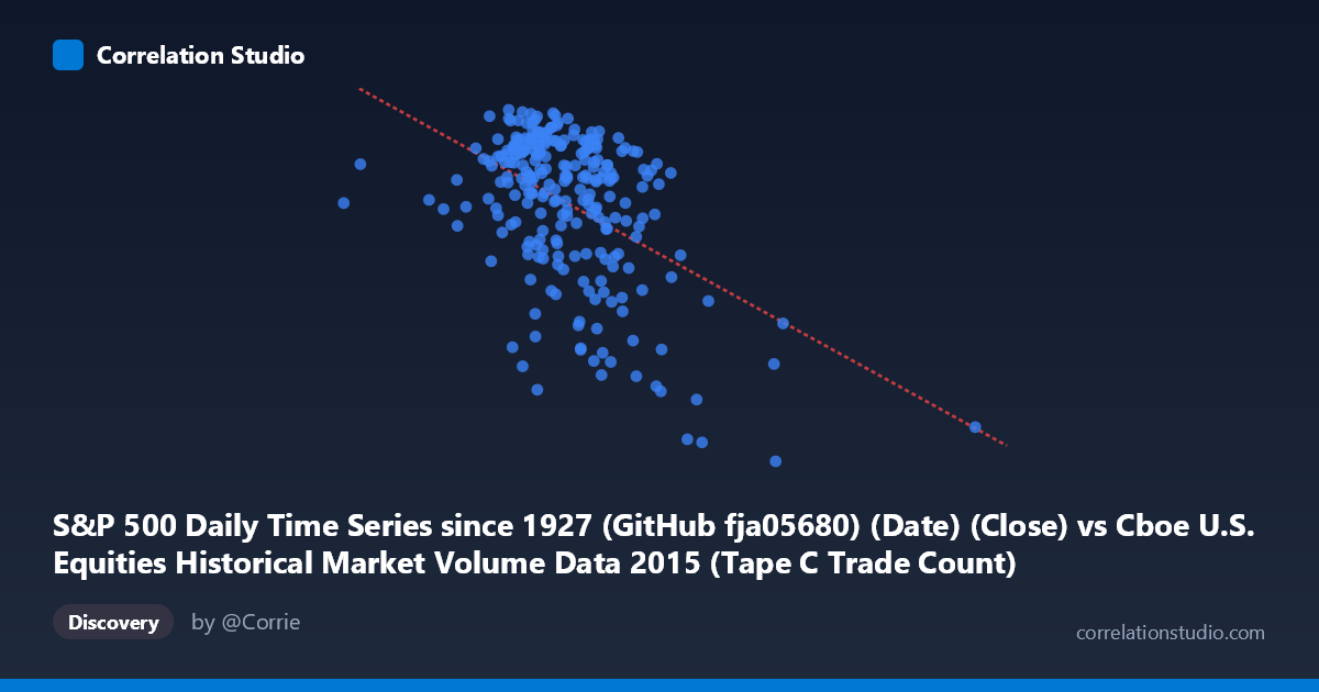
S&P 500 Daily Time Series since 1927 (GitHub fja05680) (Date) (Close) vs Cboe U.S. Equities Historical Market Volume Data 2015 (Tape C Trade Count)

Pearson correlation (r): -0.474
Spearman correlation: -0.3623
p-value: 0
Sample size (n): 252
95% confidence interval: -0.5645 to -0.3722
Granger causality: None
Granger optimal lag: 1

AI analysis

Analysis: S&P 500 Close Price vs. Cboe Tape C Trade Count (2015)

Relationship Overview The scatterplot reveals a moderate negative relationship between the S&P 500 daily closing price (X-axis) and the Cboe Tape C trade count (Y-axis) across 2015 trading days. As the S&P 500 index level increases, the number of trades in Tape C (NYSE-listed securities) tends to decrease. The linear regression equation (y = −0.000197x + 2,210.68) quantifies this inverse slope, meaning that for every 100,000-point increase in the index close, trade count falls by approximately 19.7 units — a modest but consistent directional signal visible across the point cloud.

Correlation Strength and Statistical Significance The Pearson correlation of r = −0.474 indicates a moderate negative association, but the variance explained metric tells the more important story: R² = 0.2247, meaning only about 22.5% of the variance in Tape C trade counts is explained by the S&P 500 close price. Roughly 77.5% of the variation in trading activity is driven by factors not captured here. The 95% confidence interval of [−0.565, −0.372] is meaningfully below zero throughout, and the p-value of 1.55×10⁻¹⁵ confirms this is not a chance finding given n = 252 paired observations from a population of 3,302. However, the Granger causality tests are entirely non-significant in both directions (X→Y: F = 0.079, p = 0.779; Y→X: F = 0.355, p = 0.552), meaning that neither variable temporally predicts the other at a one-period lag. This is a critical caveat: the correlation reflects a contemporaneous co-movement — likely both being driven by shared market conditions — rather than any directional predictive or causal mechanism.

Notable Patterns, Clusters, and Outliers The data exhibits a clear bifurcation or clustering structure that deserves attention. The bulk of observations concentrate in the X range of roughly 600,000–900,000 with Y values between ~2,040–2,130, forming a dense central cloud with relatively modest negative slope. However, a distinct lower-right cluster emerges at higher X values (≥950,000–1,200,000+) with noticeably depressed trade counts (Y ≈ 1,867–1,970). Points like (1,194,527, 1,867.61) and (1,040,483, 1,881.77) are conspicuous low-Y outliers at high X values. There is also a left-tail outlier at (291,078, 2,060.99) — an unusually low volume day with an average trade count — which appears isolated from the main cluster. This bimodal-like separation suggests the relationship may not be strictly linear and could reflect distinct market regimes within 2015 (e.g., calm trending periods vs. volatile, high-volume episodes).

Confounding Factors and Interpretive Caveats Several important confounds complicate interpretation. First, both variables are time-indexed to 2015, meaning macroeconomic events (the August 2015 flash crash, Fed rate decision uncertainty, China volatility) likely drive both the index level and trading activity simultaneously — a classic spurious correlation via shared external driver. Second, the S&P 500 close price itself is a cumulative price level, not a return, so its range over a single year is relatively compressed; this means the correlation partly reflects time-of-year trends (e.g., market drifting higher through mid-year while routine trading volumes declined, then spiking in volatility periods). Third, Tape C specifically covers NYSE-listed securities, not the full market, so it may respond to exchange-specific structural factors (routing, market share shifts) independent of index performance. Finally, the Granger causality result at only lag-1 may miss longer-horizon dynamics; a multi-lag analysis could reveal different patterns.

Actionable Insights and Further Investigation Practitioners should not use the S&P 500 price level alone as a predictor of Tape C trading activity, given the weak explained variance and absent Granger causality. More productive avenues include: (1) incorporating VIX or realized volatility alongside price level, as fear and uncertainty are well-known trading activity amplifiers; (2) testing non-linear models (e.g., piecewise regression or regime-switching) to better capture the apparent clustering at high-volume, low-price versus low-volume, high-price regimes; (3) extending the Granger causality test to lags 2–5 to check for longer-horizon predictive relationships; and (4) controlling for day-of-week and seasonal effects, as trade counts are known to follow calendar patterns. The August 2015 outlier cluster in particular warrants isolation as a separate regime to determine whether the negative correlation holds outside of stress periods.

X dataset: Cboe U.S. Equities Historical Market Volume Data 2015

Y dataset: S&P 500 Daily Time Series since 1927 (GitHub fja05680) (Date)

Part of experiment: Daily - Cboe U.S. Equities Historical Market Volume Data 2015 vs S&P 500 Daily Time Series since 1927 (GitHub fja05680) (Date)