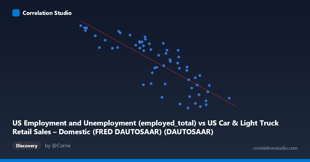
US Employment and Unemployment (employed_total) vs US Car & Light Truck Retail Sales – Domestic (FRED DAUTOSAAR) (DAUTOSAAR)
- Pearson correlation (r)
- -0.816
- Spearman correlation
- -0.8556
- p-value
- 0
- Sample size (n)
- 59
- 95% confidence interval
- -0.8868 to -0.7078
- Granger causality
- None
- Granger optimal lag
- 10
AI analysis
Scatterplot Analysis: US Domestic Auto Sales vs. Total Employment
Overview of the Relationship
The scatterplot reveals a moderately strong negative relationship between US domestic auto retail sales (X-axis, measured as seasonally adjusted annual rate) and total US employment (Y-axis). As domestic auto sales increase, total employment tends to decrease — a counterintuitive finding at first glance, but one that likely reflects underlying structural and temporal shifts in the US economy over the 1967–2025 time coverage. The linear regression equation (y = −10,704.9x + 188,766) captures this downward slope, with the data points showing reasonable but imperfect adherence to the trend line, suggesting meaningful scatter around the central tendency.
Correlation Strength, Direction, and Statistical Significance
The Pearson correlation of r = −0.816 indicates a strong negative association, and the R² of 0.666 means that approximately 66.6% of the variance in employment is statistically explained by variation in domestic auto sales — a substantial proportion for macroeconomic data. The 95% confidence interval of [−0.887, −0.708] is relatively tight and lies entirely in negative territory, reinforcing that this inverse relationship is not an artifact of sampling variability. The p-value of 3.55 × 10⁻¹⁵ is extraordinarily small, making the correlation highly statistically significant and effectively ruling out chance as an explanation. However — and critically — the Granger causality tests fail in both directions (X→Y: F = 0.99, p = 0.47; Y→X: F = 1.74, p = 0.12). Neither variable temporally predicts the other at the optimal 10-period lag, meaning this strong correlation carries no detectable directional forecasting power. This is a decisive caveat: statistical association does not imply that auto sales drive employment levels or vice versa.
Notable Patterns, Clusters, and Outliers
Several structural features are visible in the data. There is a loose cluster of high-employment, low-sales observations in the lower-right region (e.g., points near X ≈ 8.5–10.1, Y ≈ 74,000–100,000), which likely corresponds to periods of elevated auto production activity coinciding with pre-restructuring eras or post-recession recovery phases in the auto industry. Conversely, points in the upper-left (X ≈ 1.9–3.5, Y ≈ 139,000–163,000) represent high-employment periods with suppressed domestic auto sales — plausibly reflecting recent decades when employment grew but domestic auto market share shifted toward imports and foreign-branded vehicles. A few potential outliers stand out: the point at (1.86, 163,493) sits at the extreme upper-left and likely reflects a recent high-employment, low-domestic-sales environment. The point at (10.14, 85,064) at the far right suggests a historical era of peak domestic auto sales but comparatively lower total employment. The scatter also hints at mild non-linearity, with the relationship potentially flattening or curving at the extremes.
Confounding Factors and Interpretive Caveats
The most important caveat is that this is almost certainly a spurious or indirect correlation driven by long-term secular trends rather than a direct causal mechanism. Over the 58-year window (1967–2025), both variables have followed independent structural trajectories: domestic auto sales have generally declined as import penetration and SUV/light truck classifications shifted market composition, while total employment grew substantially with population expansion and labor force participation changes. This creates a time-trend confound — two variables can correlate strongly simply because they both trend over decades without any meaningful causal link. The annual aggregation of employment data paired with monthly auto sales also introduces temporal mismatch. Additionally, the negative direction seems economically paradoxical (more jobs should support more purchases), which itself signals that a third variable — likely time or structural economic change — is the true driver of the observed pattern.
Actionable Insights and Further Investigation
Given the absence of Granger causality, practitioners should avoid using domestic auto sales as a leading indicator of employment (or vice versa) in forecasting models. A more productive analytical path would involve detrending both series (e.g., using first differences or HP filtering) to isolate cyclical rather than secular co-movement, then re-testing correlation and causality. It would also be valuable to disaggregate employment by sector — particularly manufacturing and auto-related employment — which would be far more theoretically linked to domestic auto sales volumes than aggregate total employment. Controlling for import market share, consumer credit conditions, and GDP growth as covariates in a multivariate regression would help isolate whether any genuine relationship persists once confounds are removed. Finally, testing for structural breaks around major events (1973 oil shock, 2008–09 financial crisis, 2020 pandemic) could reveal whether the correlation is regime-dependent rather than stable across the full time series.
X dataset: US Car & Light Truck Retail Sales – Domestic (FRED DAUTOSAAR)
Y dataset: US Employment and Unemployment
Part of experiment: Yearly - US Car & Light Truck Retail Sales – Domestic (FRED DAUTOSAAR) vs US Employment and Unemployment