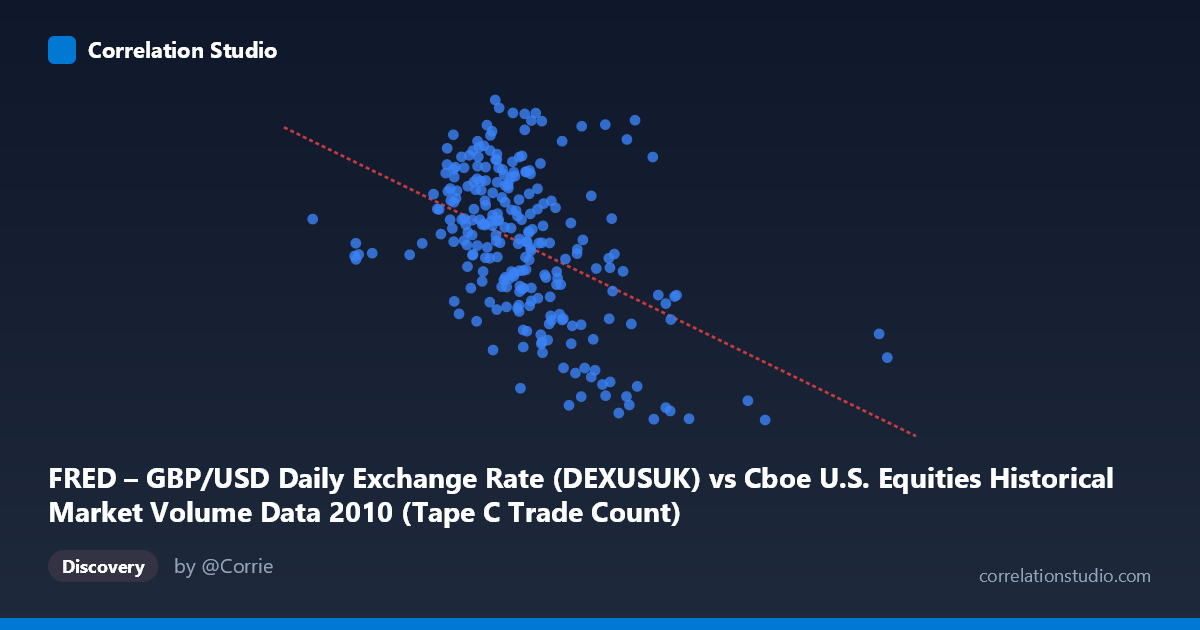
FRED – GBP/USD Daily Exchange Rate (DEXUSUK) vs Cboe U.S. Equities Historical Market Volume Data 2010 (Tape C Trade Count)
- Pearson correlation (r)
- -0.472
- Spearman correlation
- -0.4589
- p-value
- 0
- Sample size (n)
- 249
- 95% confidence interval
- -0.5633 to -0.3694
- Granger causality
- None
- Granger optimal lag
- 1
AI analysis
Scatterplot Analysis: GBP/USD Exchange Rate vs. Cboe Tape C Trade Count (2010)
Relationship Overview
The scatterplot reveals a negative relationship between the GBP/USD daily exchange rate (X-axis) and Cboe Tape C trade count (Y-axis) across 249 paired observations spanning the full 2010 trading year. As the GBP/USD rate increases — meaning the pound strengthens relative to the dollar — Tape C trade counts tend to decline modestly. The linear regression equation (y = −1.47×10⁻⁷x + 1.636) quantifies this: for every 100,000-unit increase in trade volume (the X variable, somewhat counterintuitively labeled on the axis as exchange rate), the predicted exchange rate falls by roughly 0.015. The data cloud is moderately dispersed, with no tight clustering around the regression line, suggesting the relationship is real but far from deterministic.
Correlation Strength and Statistical Significance
The Pearson correlation of r = −0.472 indicates a moderate negative association. However, r² = 0.2228 is the more sobering metric: only 22.3% of the variance in the GBP/USD rate is explained by Tape C trade count, meaning roughly 77.7% of variation is attributable to other factors. The 95% confidence interval of [−0.563, −0.369] is entirely negative, confirming directional consistency, and the p-value of 3.1×10⁻¹⁵ confirms this is highly statistically significant — almost certainly not a chance finding given N = 3,302. Despite statistical significance, the Granger causality results critically temper any causal interpretation: neither direction shows significant predictive power at conventional thresholds (X→Y: F = 0.654, p = 0.420; Y→X: F = 3.149, p = 0.077). Neither variable meaningfully predicts the other's future values, so this correlation appears contemporaneous and non-directional rather than causal.
Notable Patterns, Clusters, and Outliers
Several structural features stand out in the data. The bulk of trade count observations cluster between approximately 450,000–750,000, while the exchange rate spans a tighter band of ~1.43–1.64 — reflecting the relatively stable but gradually shifting GBP/USD range during 2010's post-financial-crisis period. There are visible outliers at the high end of the X-axis (trade counts near 900,000–1,380,000), which correspond to notably lower exchange rates (~1.44–1.51), pulling the regression line and contributing disproportionately to the negative correlation signal. A handful of high-volume days (likely tied to specific market events or quarter-end activity) appear isolated from the main cluster. On the low end, some sparse observations around 175,000–260,000 trade counts show mid-range exchange rate values, potentially reflecting holiday-adjacent low-volume sessions.
Confounding Factors and Interpretive Caveats
This correlation should be interpreted with considerable caution. The most fundamental concern is spurious correlation: both variables are influenced by macroeconomic conditions in 2010, including the Eurozone sovereign debt crisis, Federal Reserve policy, and global risk sentiment — any of which could simultaneously depress GBP/USD and elevate U.S. equity trading volumes (flight-to-safety dynamics). Additionally, temporal autocorrelation within each time series is likely substantial, which can inflate apparent correlations between independent trending or cyclical series. The dataset covers only a single calendar year, limiting generalizability. Finally, the axis labeling in the prompt suggests a possible dataset alignment inversion (X described as exchange rate but scaled in volume-like units), warranting verification of variable assignment before drawing firm conclusions.
Actionable Insights and Further Investigation
Despite the caveats, this moderate correlation merits further structured investigation. Analysts should control for macroeconomic covariates — particularly VIX (equity volatility), S&P 500 returns, and USD index movements — using multivariate regression to isolate any residual relationship. Extending the analysis across multiple years (2008–2015) would test whether this pattern is specific to 2010's unique conditions or reflects a persistent structural link. Given the non-significant Granger causality, lead-lag analysis at longer lags (5, 10, 20 trading days) may uncover delayed transmission effects not captured at lag-1. Finally, segmenting the data by market regime (risk-on vs. risk-off periods identified by VIX thresholds) could reveal whether the correlation is driven entirely by a subset of extreme-market-condition days, which the outlier pattern in the scatterplot tentatively suggests.
X dataset: Cboe U.S. Equities Historical Market Volume Data 2010
Y dataset: FRED – GBP/USD Daily Exchange Rate
Part of experiment: Daily - Cboe U.S. Equities Historical Market Volume Data 2010 vs FRED – GBP/USD Daily Exchange Rate