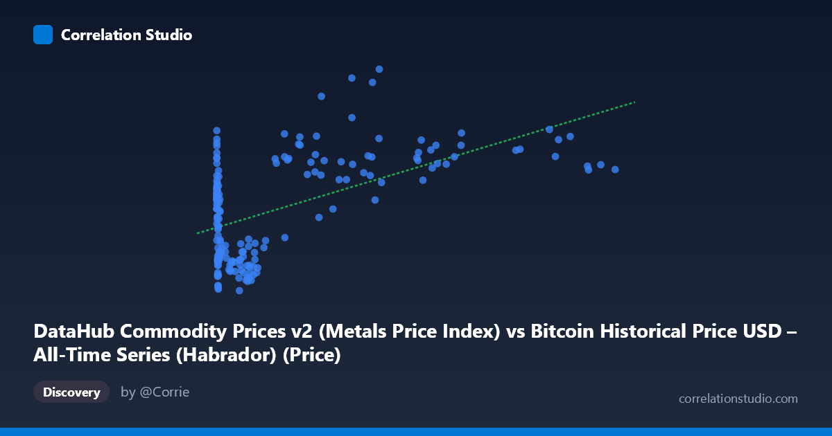
DataHub Commodity Prices v2 (Metals Price Index) vs Bitcoin Historical Price USD – All-Time Series (Habrador) (Price)
- Pearson correlation (r)
- 0.5556
- Spearman correlation
- 0.3297
- p-value
- 0
- Sample size (n)
- 182
- 95% confidence interval
- 0.4462 to 0.6486
- Granger causality
- None
- Granger optimal lag
- 1
- Time coverage
- 2010-08-01 to 2025-09-01
AI analysis
Analysis: Bitcoin Price vs. Metals Price Index
1. What the Visualization Reveals
The scatterplot shows a positive but noisy relationship between Bitcoin's historical USD price (X-axis, spanning an enormous range from $0.06 to $113,500) and a Metals Price Index (Y-axis, ranging narrowly from 92.10 to 158.57). The extreme skew in the X variable—driven by Bitcoin's exponential growth over its history—means the data is heavily concentrated at low values, with a long tail of high-price observations from more recent years. This creates a natural log-like clustering pattern rather than a clean linear spread.
2. Strength, Direction, and Uncertainty
The correlation coefficient (r = 0.556) indicates a moderate positive relationship, but r² = 0.309 reveals that only about 31% of the variance in the metals index is explained by Bitcoin's price—leaving nearly 70% unexplained by this single variable. The 95% confidence interval [0.446, 0.649] is reasonably tight and excludes zero, and the p-value (4.44E-16) confirms this correlation is highly statistically significant and not due to chance, given the sample size (n=182). However, statistical significance here reflects the strength of the trend and volume of data, not necessarily practical predictive power—31% variance explained leaves substantial room for other drivers.
Critically, the Granger causality tests show no significant predictive direction in either direction (X→Y: p=0.356; Y→X: p=0.979). This is an important caveat: despite the correlation, neither variable is a statistically useful leading indicator of the other at a 1-period lag. This suggests the relationship is better explained as a shared co-movement with broader macroeconomic trends (e.g., inflation, USD strength, or general asset market cycles) rather than one asset causally driving the other.
3. Notable Patterns and Outliers
Several features stand out: - Early-history clustering: Numerous points near X≈0–1000 (Bitcoin's early years) show Y values scattered widely (92–136), indicating high metals-index variability when Bitcoin was cheap and immature as an asset. - Non-linear/saturating trend: At high X values ($40,000), Y doesn't scale proportionally—prices like $44,354 and $46,281 correspond to Y values as high as 154–158, but similarly high X values like $105,620 and $97,365 produce lower Y (129 and 137). This suggests the relationship weakens or becomes non-monotonic at Bitcoin's highest price tiers. - Potential outlier cluster: Mid-range Bitcoin prices (~$38,000–46,000) show some of the highest Y values in the dataset (154–158), hinting at a specific time period (likely 2021-2022) where both asset classes rallied together, disproportionately influencing the regression slope.
4. Confounding Factors and Caveats
This correlation is likely confounded by time itself—both Bitcoin and metals prices have trended upward over the 2010–2025 window due to broad macroeconomic forces (monetary inflation, dollar depreciation, post-2020 stimulus-driven asset inflation). This is a classic case of spurious correlation risk via co-trending non-stationary time series. The lack of Granger causality reinforces this: rather than one market leading the other, both may be independently drifting upward due to a shared underlying factor (e.g., global liquidity conditions). Additionally, the linear regression (R²=0.309) may be a poor fit given Bitcoin's price data spans multiple orders of magnitude—a log transformation of X would likely be more appropriate and could reveal a different relationship strength.
5. Actionable Insights and Next Steps
1. Re-run analysis using log(Bitcoin price) rather than raw price, since the current linear model is likely distorted by extreme scale differences. 2. Test for cointegration (e.g., Engle-Granger or Johansen test) rather than relying on simple correlation, given both series are trending and non-stationary—this would clarify if there's a genuine long-run equilibrium relationship. 3. Introduce a control variable, such as a broad inflation measure (CPI) or USD index (DXY), to test whether the Bitcoin-metals correlation disappears once shared macro drivers are accounted for. 4. Given the absence of Granger causality, avoid using one series to forecast the other in trading or economic models; instead, treat both as co-dependent outputs of a common macro environment. 5. Segment the analysis by market regime/time period (e.g., pre-2017, 2017–2021, 2021–2025) to check if the correlation strength is stable or driven by a specific bull-market era, which the scatter pattern suggests may be the case.
X dataset: Bitcoin Historical Price USD – All-Time Series (Habrador)
Y dataset: DataHub Commodity Prices v2
Part of experiment: Bitcoin - Bitcoin Historical Price USD – All-Time Series (Habrador) vs DataHub Commodity Prices v2