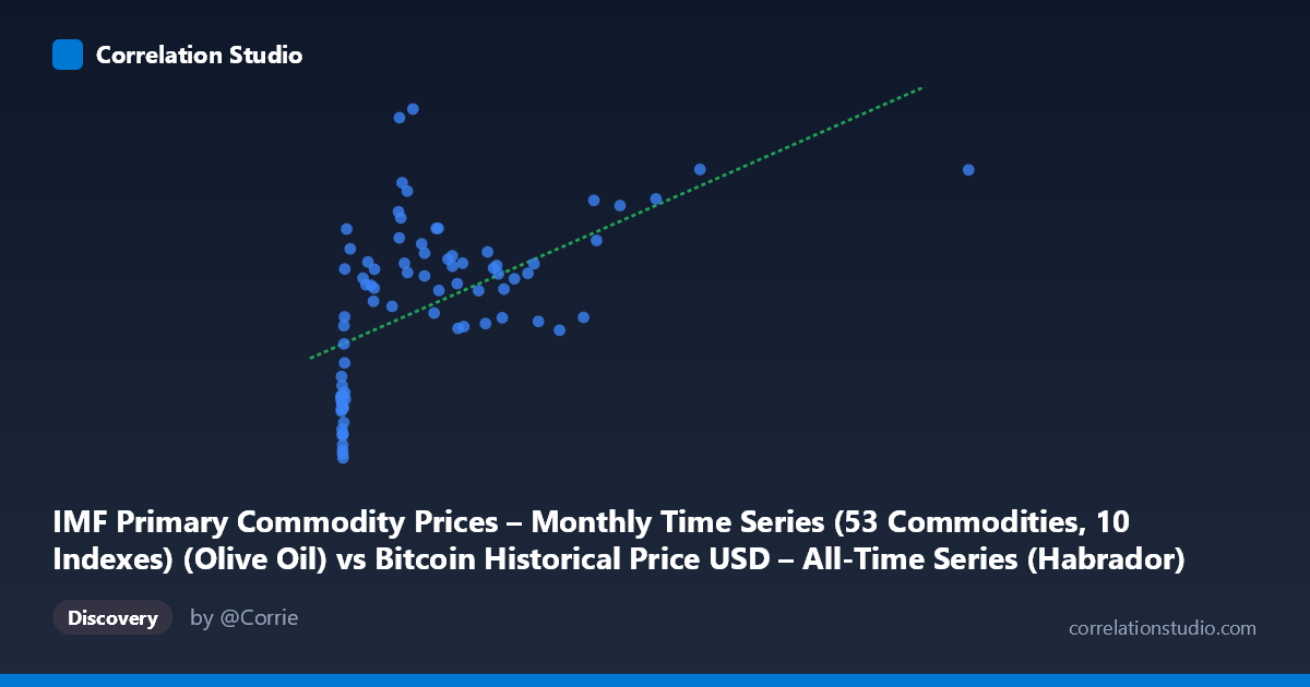
IMF Primary Commodity Prices – Monthly Time Series (53 Commodities, 10 Indexes) (Olive Oil) vs Bitcoin Historical Price USD – All-Time Series (Habrador) (Price)
- Pearson correlation (r)
- 0.5557
- Spearman correlation
- 0.6695
- p-value
- 0
- Sample size (n)
- 83
- 95% confidence interval
- 0.3863 to 0.6888
- Granger causality
- None
- Granger optimal lag
- 10
AI analysis
Analysis: Olive Oil Price Index vs. Bitcoin Price
1. Overview of the Relationship
The scatterplot displays a moderate positive association between the IMF olive oil price index (X) and Bitcoin's historical USD price (Y). Points cluster heavily at low X-values (under 250), with Y-values ranging widely from ~2,700 to ~5,000, and a sparser tail of higher X-values (up to 2,452) corresponding to higher Bitcoin prices (4,400–4,700 range). The overall shape suggests a rising trend, but with substantial scatter, especially in the dense low-X cluster.
2. Strength, Direction, and Statistical Confidence
The Pearson correlation (r = 0.556) indicates a moderate positive linear relationship, with r² = 0.309 meaning only about 31% of Bitcoin's price variance is statistically associated with olive oil price movements — leaving roughly 69% unexplained by this single variable. The 95% CI [0.386, 0.689] is reasonably tight and excludes zero, and the p-value (4.95E-08) confirms the correlation is highly unlikely to be due to chance in this sample. However, statistical significance should not be conflated with practical predictive power or causation. Critically, the Granger causality tests show no significant predictive direction in either direction (X→Y p=0.45; Y→X p=0.53) at the optimal lag of 10 periods. This strongly suggests the correlation is contemporaneous or coincidental rather than reflecting any temporal lead-lag mechanism — neither series meaningfully forecasts the other over time.
3. Notable Patterns and Features
The data shows a dense cluster of points where X < 50 spanning nearly the full Y range (2,700–4,500), indicating high Y-variability at low X — a sign of a possible non-linear or heteroscedastic relationship rather than a clean linear one. As X increases beyond ~600, Y values trend upward more consistently (clustering in the 3,900–4,700 range), suggesting the relationship may strengthen or straighten out only at higher X values. The note that Spearman ρ exceeds Pearson r supports this: a monotonic but non-linear (e.g., logarithmic or power-law) fit likely describes the data better than the straight line y = 0.769x + 3,443.81. No extreme outliers are apparent, but the low-X cluster's vertical spread effectively caps how well any single-variable model can perform.
4. Confounding Factors and Caveats
This is very likely a spurious correlation driven by shared temporal trends rather than an economically meaningful relationship. Both series span 2010–2017, a period during which Bitcoin experienced dramatic secular growth (from cents to thousands of dollars) independent of commodity markets, while olive oil prices follow agricultural supply/demand cycles. Any two upward-trending time series over the same period can show spurious correlation due to shared drift, especially with autocorrelated data (common in both financial and commodity price series) — this inflates r without indicating a causal or mechanistic link. The small sample size (n=83 paired points from a population of 449) and lack of Granger causality further undermine confidence in a genuine directional relationship. Sampling design (every 1st point) and potential temporal misalignment between monthly commodity data and continuous Bitcoin price data are additional data-quality concerns.
5. Recommendations for Further Investigation
Given the lack of Granger causality and the likely non-linear/spurious nature of the relationship, analysts should: (1) detrend both series (e.g., using differencing or log-returns) and re-test correlation to control for shared time trends; (2) test non-linear model fits (log, polynomial) as suggested by the Spearman-Pearson discrepancy; (3) treat this pairing primarily as a statistical curiosity rather than an actionable trading/economic signal, since no predictive mechanism links olive oil prices to Bitcoin; and (4) if genuine interest exists in commodity-crypto relationships, consider testing against more theoretically-grounded assets (e.g., gold, energy prices) with proper cointegration testing rather than raw correlation.
X dataset: Bitcoin Historical Price USD – All-Time Series (Habrador)
Y dataset: IMF Primary Commodity Prices – Monthly Time Series (53 Commodities, 10 Indexes)
Part of experiment: Bitcoin - Bitcoin Historical Price USD – All-Time Series (Habrador) vs IMF Primary Commodity Prices – Monthly Time Series (53 Commodities, 10 Indexes)