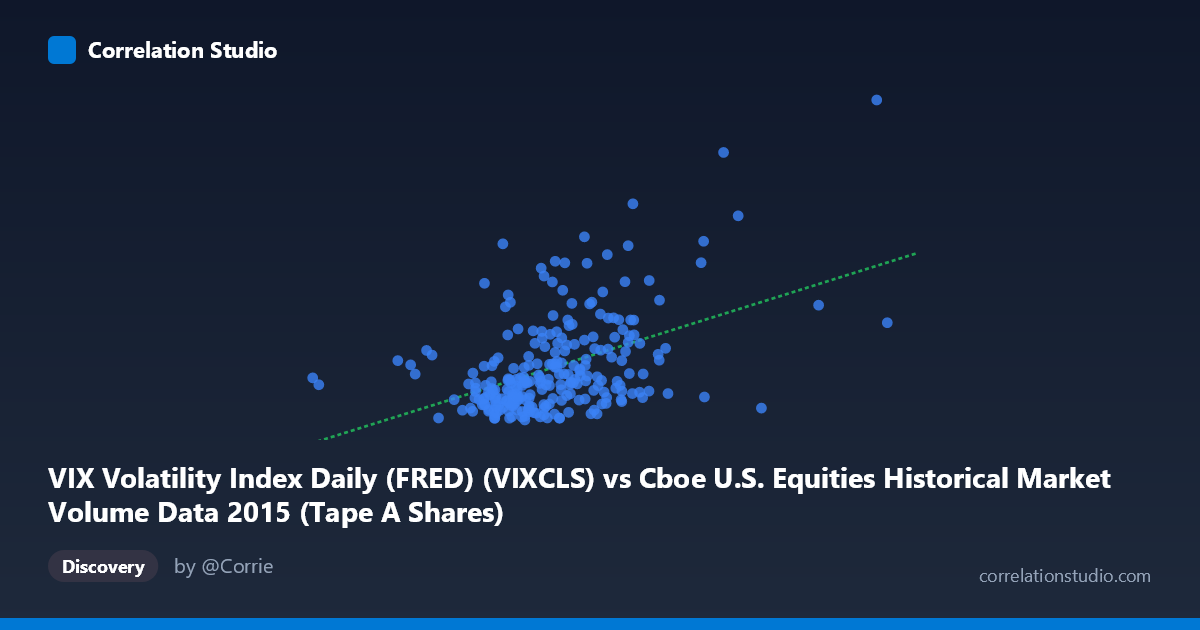
VIX Volatility Index Daily (FRED) (VIXCLS) vs Cboe U.S. Equities Historical Market Volume Data 2015 (Tape A Shares)
- Pearson correlation (r)
- 0.4589
- Spearman correlation
- 0.4052
- p-value
- 0
- Sample size (n)
- 252
- 95% confidence interval
- 0.3555 to 0.5512
- Granger causality
- None
- Granger optimal lag
- 1
- Time coverage
- 2015-01-02 to 2015-12-31
- Recomputed on refreshed data
- 2026-10-21 (r was 0.4589)
AI analysis
Analysis: VIX Volatility Index vs. Cboe U.S. Equities Market Volume (Tape A Shares) — 2015
1. Overall Relationship
The scatterplot reveals a moderate positive relationship between daily U.S. equities market volume (measured in notional value, X-axis) and the VIX Volatility Index closing values (Y-axis) across 2015. The linear regression equation (y = 3.97E-08x + 5.57) confirms that as trading volume increases, VIX tends to rise as well — a relationship that is financially intuitive, since periods of market stress and elevated fear typically drive both higher implied volatility and heavier trading activity. The cloud of points shows a generally upward-sloping trend, though with considerable scatter, suggesting the relationship is real but far from deterministic.
2. Correlation Strength and Statistical Significance
With r = 0.4589, the correlation is moderate in magnitude and positive in direction, but the explanatory power is notably limited: r² = 0.2106 means that only about 21% of the variance in VIX is explained by trading volume, leaving roughly 79% attributable to other factors. The 95% confidence interval for r [0.3555, 0.5512] is reasonably narrow given the sample size (n = 252), indicating stable estimation, and the p-value of 1.58E-14 confirms the relationship is highly statistically significant — almost certainly not due to chance across a population of N = 3,302. However, the Granger causality analysis tells a critical story: neither direction of temporal predictability is significant (X→Y: F = 0.0014, p = 0.97; Y→X: F = 0.467, p = 0.50). This means that knowing yesterday's volume does not help predict today's VIX, and vice versa — the two variables move together contemporaneously rather than one leading the other. This is a crucial caveat for any trading or risk management strategy that might attempt to use one as a leading indicator of the other.
3. Notable Patterns, Clusters, and Outliers
Several features stand out in the data distribution:
- A dense core cluster exists roughly between X = 220M–300M and Y = 12–20, representing the "normal" regime of 2015 trading conditions where volume and VIX were relatively contained. - A clear upper-right scatter of high-volume, high-VIX points is visible, likely corresponding to the August 2015 market selloff, when the VIX spiked dramatically (sample points reaching Y = 36.02 and Y = 28.03) alongside surging volume (X values approaching 400M+). The point at approximately (401M, 36.02) is a pronounced outlier and likely represents a single extreme stress day. - Low-VIX, moderate-volume points cluster at the bottom (Y ≈ 12–14), suggesting a floor in VIX behavior even when volume is average — consistent with VIX's known mean-reverting properties. - The relationship appears to exhibit heteroscedasticity: variance in VIX increases substantially at higher volume levels, suggesting the linear model may underfit the upper tail of the distribution.
4. Confounding Factors and Caveats
Several important caveats temper interpretation:
- Reverse causality ambiguity: While Granger tests show no lag-based prediction, contemporaneous causality is unresolved — market fear (VIX) may drive volume, volume may drive VIX, or both may be jointly driven by external news shocks (e.g., China slowdown fears in August 2015, Federal Reserve rate decision uncertainty). - Event clustering: The August 2015 volatility episode likely disproportionately drives the correlation. Removing those ~20 extreme days could substantially reduce r, making the relationship an artifact of a single market episode rather than a stable structural relationship. - VIX is forward-looking (30-day implied volatility), while volume is a contemporaneous measure — they operate on different temporal horizons, which the Granger analysis implicitly reflects. - Tape A Shares specificity: Using only Tape A (NYSE-listed securities) may not fully represent total market stress signals captured by the VIX, which is S&P 500-based. - Seasonality and calendar effects in 2015 volume patterns (e.g., lower summer volume, year-end effects) may create spurious correlation with VIX's own seasonal tendencies.
5. Actionable Insights and Further Investigation
- Regime-based analysis is strongly recommended: segment the data into low-VIX (< 15), medium-VIX (15–25), and high-VIX ( 25) regimes and re-examine correlations separately. The relationship may be non-linear or regime-dependent, with much stronger coupling during stress episodes. - Outlier sensitivity analysis: Re-run the correlation excluding the August 2015 spike period to determine whether the r = 0.46 reflects a structural relationship or is largely event-driven. - Non-linear modeling: Given the apparent heteroscedasticity and potential exponential behavior in the upper tail, explore log-transforming volume or fitting a piecewise/spline regression to better capture the true functional form. - Expand the temporal scope: A single calendar year (2015) is a narrow window. Testing whether this correlation holds across multiple years would establish whether this is a durable market microstructure relationship or a 2015-specific phenomenon. - Cross-instrument validation: Compare Tape B and Tape C volume alongside VIX to determine whether the relationship is specific to NYSE-listed equities or a broader market-wide phenomenon.
X dataset: Cboe U.S. Equities Historical Market Volume Data 2015
Y dataset: VIX Volatility Index Daily (FRED)
Part of experiment: Daily - Cboe U.S. Equities Historical Market Volume Data 2015 vs VIX Volatility Index Daily (FRED)