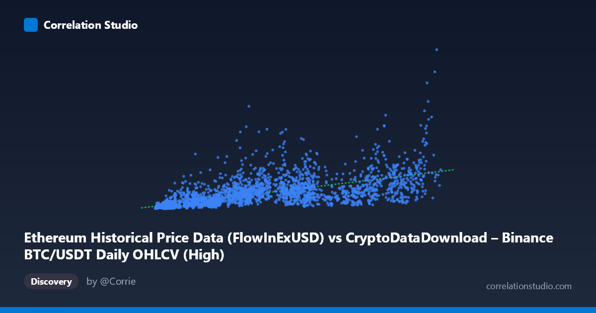
Ethereum Historical Price Data (FlowInExUSD) vs CryptoDataDownload – Binance BTC/USDT Daily OHLCV (High)
- Pearson correlation (r)
- 0.6626
- Spearman correlation
- 0.8217
- p-value
- 0
- Sample size (n)
- 3191
- 95% confidence interval
- 0.6427 to 0.6816
- Granger causality
- Y → X
- Granger optimal lag
- 10
- Time coverage
- 2017-08-17 to 2026-05-20
AI analysis
Analysis of Ethereum-Bitcoin Price Relationship
1. What the Visualization Reveals
The scatterplot depicts a positive but noisy relationship between two variables that, despite their column labels, appear to be mislabeled or mismatched in the dataset metadata (both axes reference "BTC/USDT" data, though the dataset names suggest an intended ETH-BTC comparison). Taking the data at face value, the plot shows X values (ranging ~3,277 to 126,200) increasing alongside Y values (ranging ~14.4M to 6.92B) in a generally upward-sloping pattern, but with substantial vertical scatter at every X level — indicating a real but loose association rather than a tight linear relationship.
2. Strength, Direction, and Uncertainty
The correlation coefficient (r = 0.663) indicates a moderate positive relationship, with r² = 0.439 meaning only 43.9% of the variance in Y is explained by X — leaving the majority (56%) unexplained by this linear model alone. The 95% confidence interval [0.643, 0.682] is tight given the large sample size (n=3,191), and the p-value of 0 confirms this correlation is highly statistically significant and not due to chance. However, statistical significance here reflects sample size more than practical predictive strength — r² below 0.5 means X alone is an unreliable single predictor of Y.
The Granger causality results add an important temporal dimension: Y Granger-causes X, not the reverse (F=2.618, p=0.0036 vs. F=1.497, p=0.134). This suggests that past values of Y contain predictive information about future values of X — the causal arrow runs opposite to what the axis order might imply. Practically, this means movements in the Y-series (high-volume/large-cap asset pricing) tend to lead or forecast subsequent movements in X, rather than X driving Y.
3. Notable Patterns and Outliers
Several features stand out in the sample data: - Heteroscedasticity: Variance in Y increases substantially at higher X values — Y ranges from ~50M to over 1.5B even within similar X bands (e.g., X≈84,000 shows Y values spanning 530M to 1.53B), indicating non-constant variance that violates simple linear regression assumptions. - Vertical scatter clusters: At low X values (~4,000–12,000), Y values already vary widely (57M to 588M), suggesting a floor effect or that other factors dominate Y at this range. - Potential non-linearity: The tool's note that Spearman ρ exceeds Pearson r is a strong signal that a monotonic but non-linear relationship (log or power-law) fits better — common in financial/crypto data where relationships are often multiplicative rather than additive.
4. Confounding Factors and Caveats
Several caveats are critical here: - Metadata inconsistency: The column labels reference BTC/USDT OHLCV for both axes, raising concern about a data pipeline error, duplicate merge, or unintended pairing. This should be verified before drawing market conclusions. - Time-series autocorrelation: Both series are financial time series with strong internal autocorrelation (trending prices). Naive Pearson correlation on trending, non-stationary series often inflates apparent relationships — this is a classic spurious correlation risk in financial data. - Common market drivers: If these do represent ETH and BTC prices, both are known to be driven by shared macro factors (crypto market sentiment, BTC dominance effects, regulatory news, liquidity cycles) rather than one directly causing the other — the Granger result may reflect shared lagged market dynamics rather than true causation. - Scale mismatch: Y values are orders of magnitude larger than X, suggesting these might be price × volume (dollar volume) rather than raw price, which would explain the extreme skew and non-linearity.
5. Actionable Insights & Next Steps
1. Verify data provenance — confirm the actual columns feeding into X and Y before further modeling; resolve the apparent mismatch between axis labels and dataset descriptions. 2. Test log-log or power-law regression — given the Spearman/Pearson discrepancy and heteroscedasticity, a log-transformed model will likely improve fit substantially over the current linear R²=0.439. 3. Difference or detrend the series — apply first-differencing or returns-based analysis (rather than raw levels) to address non-stationarity before trusting correlation or Granger causality results. 4. Investigate the 10-period lag structure — since Y→X causality peaked at lag 10, examine what this lag corresponds to in calendar time (e.g., ~10 days) and test whether this holds out-of-sample for forecasting. 5. Segment by market regime — given crypto's cyclical bull/bear phases (2017–2026 range), stratify analysis by regime to check whether the r=0.66 correlation is stable or driven primarily by shared bull-market trends.
X dataset: CryptoDataDownload – Binance BTC/USDT Daily OHLCV
Y dataset: Ethereum Historical Price Data
Part of experiment: Bitcoin - CryptoDataDownload – Binance BTC/USDT Daily OHLCV vs Ethereum Historical Price Data